- Research
- Open access
- Published:
Stock market and macroeconomic variables: new evidence from India
Financial Innovation volume 5, Article number: 29 (2019)
Abstract
Understanding the relationship between macroeconomic variables and the stock market is important because macroeconomic variables have a systematic effect on stock market returns. This study uses monthly data from India for the period from April 1994 to July 2018 to examine the long-run relationship between the stock market and macroeconomic variables. The empirical findings suggest that standard cointegration tests fail to identify any relationship among these variables. However, a transformation that extracts the actual functional relationship between these variables using the alternating conditional expectations algorithm of (J Am Stat Assoc 80:580–598, 1985) identifies strong evidence of cointegration and indicates nonlinearity in the long-run relationship. Further, the continuous partial wavelet coherency model identifies strong coherency at a lower frequency for the transformed variables, establishing the fact that the long-run relationship between stock prices and macroeconomic variables in India is nonlinear and time-varying. This evidence has far-reaching implications for understanding the dynamic relationships between the stock market and macroeconomic variables.
Introduction
Understanding the relationship between macroeconomic variables and the stock market is important because macroeconomic variables have a systematic effect on stock market returns. Economic forces affect discount rates, and through this mechanism, macroeconomic variables become part of the risk factors in equity markets [Chen et al. 1986]. Arbitrage pricing theory assumes that financial stocks can be influenced by the behavior of macroeconomic fundamentals; there are many channels for the relationships between the stock market and key macroeconomic variables. For example, Friedman (1988) advocated the wealth and substitution effects to measure the relationship between the stock market and money. Moreover, three separate hypotheses have been proposed to explain the theoretical relationship between the stock market and the exchange rate: Frenkel’s (1976) asset market hypothesis, Dornbusch and Fischer’s (1980) goods market hypothesis, and Frankel’s (1983) portfolio balance hypothesis.
Studies have shown that the choice of the financial and macroeconomic variables that influence the stock market is intriguing and puzzling, and have attempted to explain the anomalous relationship through different hypotheses [Fama (1981), Geske and Richard (1983), Ram and Spencer (1983), Fama (1990), Schwert (1990), Cochrane (1991) and Lee (1992)]. Fama (1981) explained the anomalous negative correlation between inflation and real stock returns by proposing a proxy hypothesis, where the anomalous negative correlation is the result of the negative relationship between inflation and real output and the strong positive relationship between real output and real stock returns. Ram and Spencer (1983) found evidence of a positive relationship between inflation and real output, consistent with the Phillips curve hypothesis.
While many researchers provide empirical support for linear long-run relationships between stock markets and macroeconomic variables, studies like Mukherjee and Naka (1995), Cheung and Ng (1998), Binswanger (2004), Nasseh and Strauss (2000), Wongbangpo and Sharma (2002), Kizys and Pierdzioch (2009), Bekhet and Matar (2013), Inci and Lee (2014) and Lawala et al. (2018) employed Engle and Granger’s (1987) methodology to infer causal relationships and Granger’s (1988) and Johansen’s (1991) methodology for cointegration between these variables. Most of the earlier empirical studies implicitly assumed that the relationships between the stock market and macroeconomic variables are linear in nature and time-invariant. In their cointegration analyses, most of these studies failed to test the stability of the parameters over time or the asymmetric long-run relationships among these variables. Hansen and Johansen (1999) and Johansen et al. (2000) emphasized that the results of cointegration analysis are highly sensitive to sample selection and have potential parameter instability over time.
In this regard, McMillian (2005) estimated the time-varying relationships between the stock market and other macroeconomic variables for U.S. data using Johansen’s (1991) cointegration test in a rolling and recursive sample window and suggested that the long-run relationships between these variables are time varying. The main drawback of implementing a rolling or recursive cointegration is that the variables under consideration should have the same time series properties for all sample windows; if these properties change for a given subsample of windows, then the interpretations from the analysis are biased. On the other hand, a good number of recent studies have examined the nonlinear relationships between key macroeconomic variables such as output, inflation, and exchange rates, and found evidence in favor of the asymmetric behavior of these variables over a period. Studies like Falk (1986), Ramsey and Rothman (1996), and Bradley and Jansen (1997) all support various forms of nonlinear adjustment among key macroeconomic variables. In line with these findings, studies by Boucher (2007) and Kizys and Pierdzioch (2009) highlight that the relationships between the stock market and macroeconomic variables are asymmetric and these relationships will change in the long run.
The nonlinearities in financial markets are explained by many studies, such as Dumas (1992), Brock and LeBaron (1996), Sarantis (2001), Shleifer and Robert (2003), and Humpe and Macmillan (2014). These studies all identify the interaction between informed and noise traders, suggesting speculators are the main source for the market’s nonlinear behavior.
From an empirical standpoint, the functional form of any relationship should be appropriate before performing any analysis. When the relationship is nonlinear, a linear analysis may lead to misleading conclusions, with the potential of inferences that there is no relationship between the variables under consideration. Although some studies highlight the possible nonlinear relationships between the stock market and macroeconomic fundamentals, the issue has received little comprehensive attention in the empirical literature. A few studies, like Kanas (2003, 2005), Zhou (2010), and Tang and Zhou (2013), have documented nonlinear relationships for different variables, and explored the alternating conditional expectations (ACE) algorithm developed by Breiman and Friedman (1985) to identify the correct functional form and transform the variables to be used in the empirical analysis. The results from these studies show that the advantage of using the ACE algorithm is its ability to identify the exact functional form of the nonlinear relationship. Once the correct functional form of the variables has been identified, further investigation can proceed.
Recent advances in time-series econometrics have produced methodologies for analyzing the relationships between variables in a frequency domain, where the actual relationship might vary at different frequencies. For example, some studies of India have used frequency domains and wavelet analysis. Durai and Bhaduri (2009) examined the stock market and economic activity using discrete wavelets to decompose the time series of the variables into different frequencies; the results suggest that the variables are connected in different ways at different frequency levels. Tiwari et al. (2013) used the continuous wavelet transformation (CWT) developed by Conraria and Soares (2011). The advantage of the CWT over discrete wavelet transformation (DWT) is the identification of the correlation between variables in different frequencies over time scales. Even though the CWT has a major disadvantage it can be used only for two variables the concepts of wavelet multiple coherencies and partial wavelet coherency to some extent compensate, allowing the CWT to move beyond bivariate analysis.
The purpose of the present study is to extend the existing nonlinear and time-varying empirical literature to clarify the relationship between stock prices and key macroeconomic fundamentals in the Indian context. The study’s main contribution is twofold. First, the analysis of nonlinearity in the relationships between the stock market and other key macroeconomic variables for Indian data provides a developing country perspective. Second, using continuous wavelets to understand the coherency between two variables in the frequency domain for different time scales provides a better understanding than implementation of a rolling or recursive cointegration.
The remainder of the paper is organized as follows. Section 2 describes the nonlinear cointegration approach using an ACE algorithm and provides a brief outline of the CWT methodology used in the study. Section 3 describes the data, and in section 4, the results of the empirical estimation are reported. Finally, section 5 draws conclusions based on the study’s empirical findings.
Nonlinear and time-varying relationships
The conventional cointegration tests of Engel and Granger (1987) and Johansen (1991) implicitly assume linearity and time invariance. The inferences drawn from these tests may be misleading if the relationships are nonlinear and time-varying. Following McMillian (2005), this study uses a rolling cointegration test for stock prices and other macroeconomic variables. In the rolling framework, we fix the size of a rolling sample window,Footnote 1 and move the sample window by adding one observation to the end and removing the first one. For each rolling sample window, we conduct conventional augmented Dickey-Fuller (ADF) unit root tests to determine the order of integration for each of the variables used in every rolling window. If the test ensures all variables are integrated of order one in all rolling windows, then we can move to implement the conventional Johansen (1991) cointegration test and the trace statistics can be observed and scaled by their 5% critical values. The null hypothesis of no cointegration can be rejected at a 5% level for the specified sub-sample period if the value of the scaled test statistic is greater than one.
The ACE algorithm and nonlinear cointegration
The ACE algorithm
Granger and Hallman (1991) and Meese and Rose (1991) analyzed the non-parametric ACE algorithmFootnote 2 developed by Breiman and Friedman (1985) for raw variables to obtain nonlinear transformations of their respective variables and used a causality test for the transformed variables to infer a nonlinear causal relationship. The ACE method converts the original variables into transformed variables, ensuring that there is maximum correlation between the variables with the highest R-squared; ACE procedures adopt extremely weak distributional assumptions and can handle a wide variety of nonlinear transformations of the data by utilizing flexible data smoothing techniques. Thus, any test on these transformed variables can be viewed as evidence for nonlinearity.
Assume a linear regression model contains k independent variables, namely x1t, x2t, …., and xkt, and a dependent variable yt:
Where, δ0, δ (i = 1,2,…,k) are the regression coefficients to be estimated, and εt is an error term. Thus eq. (1) assumes that yt, the dependent variable, is a linear function of k independent variables. An ACE algorithm using the regression model in eq. (1) can be written as.
Where f is a function of the dependent variable y, and ni is a function of the independent variables xi (i = 1,2,…,k). Equation (2) shows f (·), n1 (·), n2 (·) …, and nk (·) is the optimal transformation to be estimated. The ACE regression normalizes the coefficients to unity.
The ACE algorithm initially starts by defining arbitrary determinate mean zero transformations, f (yt), n1(x1t), n2(x2t),. ., and nk (xkt). To obtain the optimal transformation, the estimated model ensuring the maximum correlation among the variables and highest R-square from a regression as specified in eq. (2). Under the constraint of E [f (yt)]2 = 1, this is equivalent to minimizing the expected mean squared error of the regression. The expected mean squared error is given by
Minimization of u2 with respect to ni (xi) (i = 1,2,…,k) and f(yt) is carried out through a series of single-function minimizations, resulting in the following equations:
With \( \left\Vert \bullet \right\Vert \equiv {\left[E{\left(\bullet \right)}^2\right]}^{\frac{1}{2}} \)
The algorithm involves two basic mathematical operations: conditional expectations and iterative minimization; thus, the transformation is referred to as alternating conditional expectations. Using eq. (4) to transform all variables, one variable is fixed and the transformation of the variable in question is estimated using a nonparametric data smoothing technique; the algorithm then continues to the next variable. For each variable, the iterations continue until the mean squared error of eq. (3) has been minimized. Breiman and Friedman (1985) show that the ACE algorithm provides transformations such that f (yt), n1(x1t), n2(x2t), …., and nk (xkt) converge asymptotically to the true functional forms of the optimal transformations. The distinction of these transformations is that ACE does not treat the explanatory variables as fixed, but instead treats the variables as drawn from a joint distribution. After the estimation of ni (xit) (i = 1,2,…,k), f (yt) is estimated, conditioned on these estimates, according to eq. (5). Alternating between Eqs. (4, 5), the ACE method iterates until eq. (3) is minimized. The transformations of ni*(xi) (i = 1,2,…,k) and f *(y) that achieve minimization are the optimal transformations.
Nonlinear Cointegration
As argued in studies like Granger (1991), Granger and Hallman (1991), Meese and Rose (1991), Kanas (2003, 2005) and Tang and Zhou (2013), nonlinear cointegration can be characterized from the linear cointegration of the ACE transformed variables. There are two steps involved in this procedure. First, as highlighted by Granger and Hallman (1991), in converting all original variables into ACE transformed variables, we have to ensure that the transformed variables do not deviate from the time-series properties of the original variables. Second, the usual Johansen (1991) type cointegration test is implemented for the transformed variables. This nonlinear cointegration can also be used in a rolling framework to examine time-varying nonlinearity in the relationship. If the transformed variables deviate from the time series properties of the original variables for the entire sample period or any subsample period in a rolling window, we cannot implement the usual cointegration test to capture the time varying aspect of the relationship. In that case, we propose using the continuous wavelet transform methodology to understand the relationship at different frequencies over time.
Continuous wavelet transform
CWT is a better alternative model for understanding the time-varying and nonlinearity of the relationships between stock prices and other macroeconomic variables. Wavelet coherency is used to determine the coherency between two variables for different frequencies over time, and partial wavelet coherency is used to determine the coherency between two variables conditional upon other variables for different frequencies over time. Following Conraria and Soares (2011), the methodology of deriving the CWT is as follows. The set of square integrables and the space of finite energy functions is denoted by L2 (R) The minimum criteria to impose on a function ψ (t)∈ L2 (R) The wavelets begin with a mother (admissible or analyzing) wavelet, which consists of a technical portion of the admissibility condition.
Cψ denotes the constant of the admissibility or analyzing constant.
The purpose of the wavelet is to provide the time frequency of localization; the wavelet localized function gives both the time and frequency domains.
ψ denotes wiggles up and down in the time axis; the CWT starts with a mother wavelet ψ, and a family ψ τ,s of “wavelet daughters” can be obtained by simply scaling and translating ψ:
where s denotes a scaling or dilation factor that controls the width of the wavelet and τ denotes the translation parameter, which controls the location of the wavelet. Wavelet scaling indicates stretching if (|s| > 1) or (|s| < 1), whereas translating it means shifting its position in time. Given a time series, x (t) ∈ L2 (R), the CWT of wavelet ψ is a function of two variables, W x:ψ (τ, s).
The time domain wavelet is given by τ, while the frequency domain is given by s. The wavelet transforms the time and frequency domains by mapping the original series into a function of τ and s; the wavelet provides concurrent information on the time and frequency domains. The procedures of wavelet and Fourier transformations are somewhat similar. However, the Fourier transformation differs from the wavelet in that it has no time localization parameter. Moreover, we have two functions, cosine and sine, instead of a wavelet function. CWT may also be represented in the frequency as
To develop wavelet coherency, we need two more derivations: the cross-wavelet transform (XWT) and cross wavelet power (XWP). The cross wavelet transform of two times series, x(t) and y(t), was introduced by Hudgins et al. (1993) and defined as
where Wx and Wy represent the wavelet transforms of x and y, respectively. The cross-wavelet power provides a quantified indication of the similarity of power between two time series at each time and frequency and is defined as
Complex wavelet coherency
The set of two time series x(t) and y(t) describes their complex wavelet coherency:
The Wavelet Coherency is denoted as follows
Wx and Wy are the wavelet transforms of x and y, respectively, S denotes a smoothing operator in both time and scale; without smoothing, coherency would be identical across all scales and times. The partial wavelet coherency of x1 and xj (2 ≤ j ≤ p) are denoted as follows:
r1jqjis measured as the absolute value
The Squared partial wavelet coherency of xi, j
Where φ denote the p x p matrix of all the smoothed cross-wavelet spectra Sij.
Wavelet coherency is the relationship to the product of the spectrum of each series, which can be the local correlation between the time and frequency domains in the two time series. This concept definition nearly replicates the traditional correlation coefficient. Wavelet coherence provides localized correlation coefficients in time and frequency space. When no correlation measures zero coherencies between the two time series and wavelet coherency is equal to one, it shows a strong correlation between the time and frequency domains. The statistical significance of estimated wavelet coherency can be explained through Monte Carlo simulation methods. There are no positive and negative co-movements between the time series for wavelet coherency. The information on positive and negative co-movements can distinguish the lead-lag relationships between two time series through the phase of the wavelets.
Following Conaria and Soares (2011), we can define the complex partial wavelet coherency between x and y after controlling z as follows
Cxy and Rxy are complex wavelet coherency and wavelet coherency, respectively, as defined in Eqs. (12, 13). The partial wavelet coherency between x and y given z can be defined by taking the absolute value of the denominator in eq. (13). We may write the expression for partial wavelet coherency in terms of wavelet coherency as
Data
The empirical analysis is conducted using monthly data from April 1994 to July 2018, a total of 292 observations. Monthly data of the Bombay Stock Exchange (BSE) Sensex Index, Index of Industrial Production (IIP), Wholesale Price Index (WPI), Broad Money (M3), and Exchange Rate are used. The choice of the sample is determined by the fact that a consistent new series of data is available for the sample period; it also reflects the post-liberalization period. The IIP is used as a proxy for output, while the WPI is used as a measure of inflation, and Rupees per U.S. dollar is used as a measure of the exchange rate. The data are collected from the following sources: the BSE Sensex Index is collected from their website (www.bseindia.com), and other macroeconomic variables are collected from the Handbook of Statistics on Indian Economy published by the Reserve Bank of India (RBI). All variables are seasonally adjusted, and subsequent analysis is performed on the natural logarithmsFootnote 3 of these series.
Empirical results
To analyze the long-run relationships between the stock market and other key macroeconomic variables, it is necessary to perform the conventional Engle and Granger (1987) cointegration and Johansen (1991) tests. Before considering possible cointegration between these series, their orders of integration are examined using unit root tests. The standard ADF, Phillips Perron, and Kwaitkowski et al. (1992) (KPSS) unit root tests are used, and the results are presented in Table 1. The test results show that all series are non-stationary at levels and stationary at first differences.
First, we used the conventional cointegration tests of Engle and Granger (1987) and Phillips and Ouliaris (1990) to examine the cointegration between stock prices and other macroeconomic variables. In these two tests, the null hypothesis is no cointegration, so if the calculated value of the EG and Pz statistics are significant, the null of no cointegration is rejected, indicating there is cointegration among the variables. For both these tests, the optimal lag length is determined by the Akaike information criterion, and the results are presented in Table 2.
The results from Table 2 indicate both tests fail to reject the null of no cointegration between the stock market and the macroeconomic variables, showing there is no long-run relationship between these variables. To corroborate this, we used the Johansen (1991) cointegration test for the same set of variables and the results are presented in Table 3.
The results indicate that the test statistics of trace and maximum Eigen statistics are both above the critical values at the 5% significance level. Hence, we reject the null of no cointegration relationship between these variables, which means a cointegrating relationship exists between the stock market and macroeconomic variables. The Engle and Granger (1987) cointegration and Phillips and Ouliaris (1990) tests fail to reject the null of no cointegration relationship between the stock market and other macroeconomic variables; however, the Johansen (1991) cointegration test shows the presence of a long-run relationship between these variables. Inferences drawn from conventional and Johansen (1991) cointegration tests depict a contrasting result for the relationship between the stock market and other macroeconomic variables. Gonzalo and Lee (1998) established the pitfalls in Johansen type cointegration tests and highlighted that validation by the Engle-Granger cointegration test is needed to avoid the drawbacks. Since the Engle and Granger cointegration test does not validate the Johansen test results, such contrary evidence leads to further investigation of these relationships.
The scatter plots
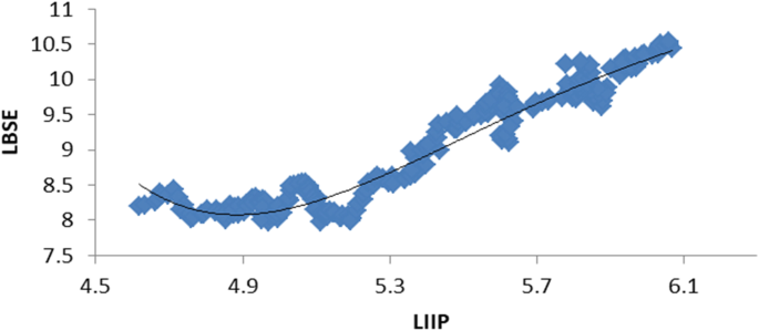
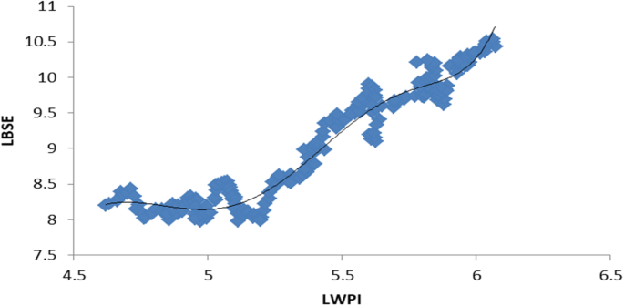
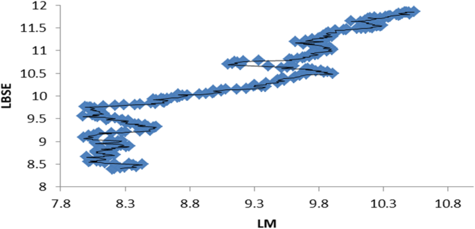
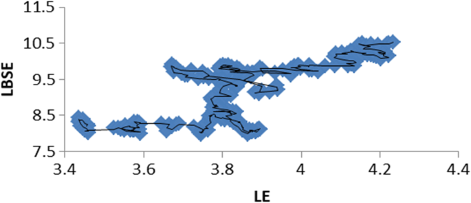
To understand these contradictory results from the two sets of cointegration tests, we need to understand the exact relationship between stock prices and each of these macroeconomic variables. A simple scatter plot of stock prices with each of these variables is depicted in Figs. 1, 2, 3, 4.
In all scatter plots, the vertical axis measures stock prices (LBSE) and all corresponding horizontal axes measure other macroeconomic variables (LIIP, LWPI, LM, and LE). These scatter plots show the nonlinear relationships between the stock market and other macroeconomic variables; moreover, the figures also show the trend lines fitted to the data. The fitted trend line for the LBSE and LIIP stands as a polynomial of order 6, whereas the trend line for LBSE and LWPI is a polynomial of order 5. For the remaining two variables, LM and LE, the trend line exhibits two and three period moving averages, respectively. Evidence from these scatter plots shows that the relationships between the stock market and other macroeconomic variables are nonlinear. This evidence restricts any linear analysis between stock prices and other macroeconomic variables in India.
To capture the nonlinearity, we employed ACE, Breiman and Friedman’s (1985) algorithm, to convert the original variables into transformed variablesFootnote 4 and test their long-run cointegration relationship. As explained, the ACE transformed variables should possess the same time series properties as the original variables, so before performing cointegration analysis, this warrants ensuring that all the transformed series retain their respective time series properties. Standard ADF, Phillips Perron, and KPSS unit root tests are used for the transformed variables to examine their stationarity. We also performed the Zivot-Andrews unit-root testFootnote 5 on the transformed series and found evidence in favor of structural breaks among the variables, which supports time variation in the relationships.
The test results in Table 4 show that all series are non-stationary at levels and stationary at first differences. Since these transformed variables possess the same properties as their original counterparts, we can now use both the conventional [Engle and Granger 1987; Phillips and Ouliaris 1990, and Johansen 1991] cointegration tests to examine the nonlinear cointegration. The results of these tests are presented in Tables 5 and 6.
The results from both conventional tests reject the null of no cointegration between stock prices and other macroeconomic variables, and accept that there is a long-run relationship between the transformed variables at conventional levels of significance. The Johansen (1991) test results also reject the null of no cointegration relationship between these transformed variables, which indicates a cointegrating relationship exists between the stock market and macroeconomic variables. Altogether, this empirical evidence suggests that long-run cointegration exists between the ACE transformed variables, which leads to the inference that there is a nonlinear cointegration between stock prices and other macroeconomic variables for the full sample period. The key implication from this evidence is that when there is a nonlinear relationship, a linear combination of the variables may lead to deceptive inferences.
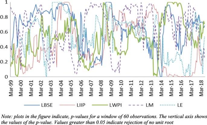
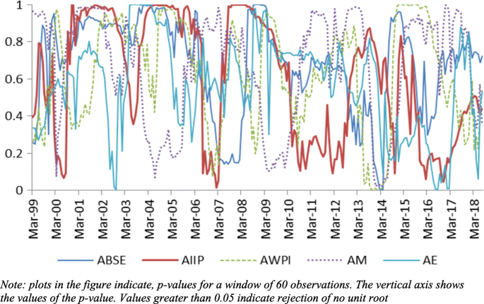
Further, regarding the possible sensitivity of the results to sample selection and parameter instability in the relationship between stock prices and other macroeconomic variables as highlighted by McMillan (2005), this study also examines the time variation in the long-run relationship between these variables using a rolling cointegration technique. Before considering the rolling cointegration test, we verify the time series properties of these variables in each subsample. In particular, the variables involved should be non-stationary in every subsample (rolling window); otherwise, the inferences might be spurious because the test statistics will be biased. Thus, we first employ rolling ADF unit root tests to check for stationarity for all series under consideration. The rolling window size is fixed at 60 observations (5 years); each time, the window is renewed by adding one observation to the end and removing the beginning observation. Thus, the first rolling window will have a sample of the first 1 to 60 observations, the second will include 2 to 61, then 3 to 62 and so on through the last observation. The test results are presented in Figs. 5 and 6.
Figure 5 clearly shows that for all the original variables (LBSE, LIIP, LWPI, LM, and LE), the null hypothesis of non-stationarity can be rejected in some sample windows, indicating that the variables change their time series properties. Similarly, Fig. 6 shows the same results for all the transformed variablesFootnote 6 (ABSE, AIIP, AWPI, AM, and AE); in some windows variables are nonstationary, while in other windows, they are stationary at the levels. Hence, we cannot implement a rolling cointegration test to identify the time-varying relationship.
To circumvent this problem, following Conraria and Soares (2011), we use CWT for both the actual and transformed variables to understand the time variation in this relationship. In this study, we concentrate only on partial wavelet coherency to determine the coherency between two variables conditional upon other variables for different frequencies over time. The main objective is to understand the relationship between stock prices and output, retaining all other variables as control variables.
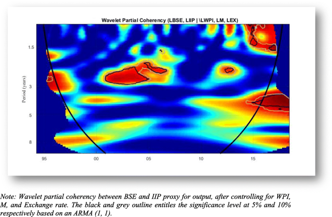
In CWT, the frequencies are split into low and high frequency, with low frequency measuring the long-run coherency between the variables and the high frequency measuring the short-run coherency. Coherency is differentiated using color codes ranging from blue to red; high coherency is indicated by the red color and the level of significance is identified with black and grey borders. Figure 7 provides the wavelet partial coherency for actual data on stock prices and output after controlling for other macroeconomic variables like inflation, money supply, and the exchange rate. The figure indicates that without transformation, there is no significant partial coherency in the low frequency, which measures the long-run partial correlation between the variables. At the high-frequency level, for some points between 2002 and 2005, there is statistically significant evidence for short-run partial coherency.
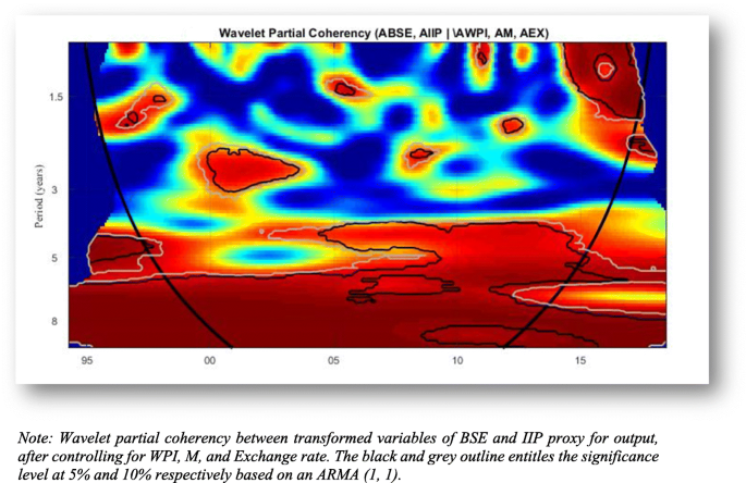
In contrast to the actual variables, Fig. 8 depicts the partial wavelet coherency for the ACE transformed variables. Like the actual data, we have analyzed the transformed stock prices and output after controlling for other transformed macroeconomic variables like inflation, money supply, and the exchange rate. The figure clearly shows a strong and significant partial coherency at a high frequency, which indicates the long-run relationship over time. The interesting inference from this analysis is that unless we identify the exact functional form of the variables, it is highly misleading to derive any plausible conclusions about their relationships. The relationships between the stock market and macroeconomic variables are nonlinearly related; if we linearly analyze and interpret them, it may result in a biased conclusion.
Conclusion
This study aimed at understanding the time-varying, nonlinear relationships between stock prices and other key macroeconomic variables using monthly data from India for the period of April 1994 to July 2018. After checking the time series properties of the variables, different cointegration tests are implemented to understand their long-run relationships. The conventional Engle and Granger (1987) and Phillips and Ouliaris (1990) tests show that there is no relationship between stock prices and other macroeconomic variables. However, the Johansen cointegration test shows that long-run relationships exist between these variables. These two contrasting results warranted further analysis. To investigate this issue, we plot simple scatter plots that indicate these variables are not linearly related, but exhibit nonlinearity.
To address the nonlinear relationships between stock prices and other macroeconomic variables, we used the ACE algorithm of Breiman and Friedman (1985). ACE algorithms identify and extract the function of these relationships by converting the original variables into ACE transformed series, which provides the functional relationships between the variables. As highlighted by Granger and Hallman (1991), nonlinear cointegration can be characterized by implementing a cointegration test for these ACE transformed variables. To do this, we must ensure that the transformed variables do not deviate from the time series properties of the original variables. All transformed series are integrated of order one at levels for the full sample period. The conventional Engle-Granger, Phillips-Ouliaris, and Johansen cointegration tests show that there is long-run cointegration between the ACE transformed variables, which indicates that a nonlinear cointegration exists between stock prices and other key macroeconomic variables for India.
To test the time-varying aspect of this relationship, we first resort to a rolling cointegration test, but the rolling unit root test for both the actual data and transformed data show changes in the behavior of time series properties in some subsample periods (rolling windows). Hence, we cannot proceed to analyze the cointegration test to identify the relationships between stock prices and other macroeconomic variables. To understand the time variation, we used the CWT method for both actual and transformed variables, and the results identify wavelet partial coherency only for the transformed variables, not for the actual variables. The inferences drawn from the CWT highlight that stock prices and other macroeconomic variables are related nonlinearly in India.
The evidence presented in this study has far-reaching implications for policymakers, researchers, and investors. Understanding the effects of macroeconomic variables on the stock market is imperative; proper comprehension of the risk and opportunities associated with macroeconomic variables may help investors make appropriate decisions based on policy reactions and help them manage the systematic risk associated with the stock market. The evidence of nonlinearity indicates the presence in the market of noise traders, arbitrage traders, and speculators and should be supported with further empirical evidence. Hence, the findings show that understanding the nonlinear relationships is an integral part of identifying the causes of different fluctuations in economic activity. As such, this study alerts financial professionals and investors to consider nonlinear empirical consistencies when modeling the stock market and macroeconomic variables.
Notes
We used different window size for testing rolling unit root and cointegration.
All the ACE transformations is derived using the package of “ace pack” in R
Variables are named LBSE (log of BSE), LIIP (log of IIP), LWPI (log of WPI), LM (log of M3) and LE (log of Exchange rate)
Once variables are ACE Transformed then named as ABSE, AIIP, AWPI, AM and AE.
Results are available upon request.
For each rolling window the ACE transformation is derived separately.
Abbreviations
- ABSE:
-
Alternating Conditional Expectation transformed Bombay Stock Exchange Sensex Index
- ACE:
-
Alternating Conditional Expectation
- ADF:
-
Augmented Dickey-Fuller
- AE:
-
Alternating Conditional Expectation transformed Exchange rate
- AIIP:
-
Alternating Conditional Expectation transformed Index of Industrial Production
- AM:
-
Alternating Conditional Expectation transformed Broad Money
- APT:
-
Arbitrage pricing theory
- AWPI:
-
Alternating Conditional Expectation transformed Whole Sale Price Index
- BSE:
-
Bombay Stock Exchange Sensex Index
- CWT:
-
Continuous wavelet transformation
- IIP:
-
Index of Industrial Production
- KPSS:
-
Kwiatkowski, Phillip, Schmidt and Shin
- LBSE:
-
Log of Bombay Stock Exchange Sensex Index
- LE:
-
Log of Exchange rate
- LIIP:
-
Log of Index of Industrial Production
- LM:
-
Log of Broad Money
- LWPI:
-
log of Whole Sale Price Index
- M3:
-
Broad Money
- RBI:
-
Reserve Bank of India
- WPI:
-
Whole Sale Price Index
References
Bekhet AH, Matar A (2013) Co-integration and causality analysis between stock market prices and their determinates in Jordan. Econ Model 35:508–514
Binswanger M (2004) How do stock prices respond to fundamental shocks? Financ Res Lett 1:90–99
Boucher C (2007) Asymmetric adjustment of stock prices to their fundamental value and the predictability of US stock returns. Econ Lett 95:339–347
Bradley M, Jansen D (1997) Nonlinear business cycle dynamics: cross-country evidence on the persistence of aggregate shocks. Econ Inq 35:495–509
Breiman L, Friedman JH (1985) Estimating transformations for multiple regression and correlation. J Am Stat Assoc 80:580–598
Brock W, LeBaron B (1996) A dynamic structural model for stock return volatility and trading volume. Rev Econ Stat 78(1):94–110
Chen NF, Roll R, Ross S (1986) Economic forces and the stock market. J Bus 59:383–403
Cheung WY, Ng LK (1998) International evidence on the stock market and aggregate economic activity, vol 5, pp 281–296
Cochrane JH (1991) Production-bases asset pricing and the link between stock return and economic fluctuations. J Financ 46:209–238
Conraria LA, Soares MJ (2011) The continuous wavelet transform: a primer, Working Paper Series NIPE WP 16/ 2011
Dornbusch R, Fischer S (1980) Exchange rates and current account. Am Econ Rev 70:960–971
Dumas B (1992) Dynamic equilibrium and the real exchange rate in a spatially separated world. Rev Financ Stud 5(2):153–180
Durai SRS, Bhaduri S (2009) Stock prices, inflation and output: evidence from wavelet analysis. Econ Model 26:1089–1092
Engle R, Granger C (1987) Co-integration and error correction representation estimation and testing. Econometrica 55:251–267
Falk B (1986) Further evidence on the asymmetric behavior of economic time series over the business cycle. J Polit Econ 94:1096–1109
Fama EF (1981) Stock returns, real activity, inflation and money. Am Econ Rev 71:545–565
Fama EF (1990) Stock returns, expected returns, and real activity. J Financ 45:1089–1108
Geske R, Roll R (1983) The fiscal and monetary linkage between stock returns and inflation. J Financ 38:1–33
Gonzalo J, Lee T-H (1998) Pitfalls in testing for long run relationships. J Econ 86:129–154
Granger C (1988) Some recent development in a concept of causality. J Econ 39:199–211
Granger CWJ (1991) Some recent generalizations of cointegration and the analysis of long-run relationships, in Long-Run Economic Relationships Oxford University Press, pp 277–287
Granger CWJ, Hallman JJ (1991) Long-memory series with attractors. Oxf Bull Econ Stat 53:11–26
Hansen H, Johansen S (1999) Some tests for parameter constancy in the cointegrating VAR. Econ J 2:25–52
Hudgins L, Friehe CA, Mayer MM (1993) Wavelet Transforms and Atmospheric Turbulence. Phys Rev Lett 71(20):3279–3283
Humpe A, Macmillan P (2014) Non-linear predictability of Stock market returns: comparative evidence from Japan and the US. Invest Manag Financ Innov 11(SSRN):4
Inci AC, Lee BS (2014) Dynamic relations between stock returns and exchange rate changes. Eur Financ Manag 20(1):71–106
Johansen S (1991) Estimation and hypothesis testing of cointegration vectors in Gaussian vector autoregressive models. Econometrica 59:1551–1580
Johansen S, Mosconi R, Nielsen B (2000) Cointegration analysis in the presence of structural brakes in the deterministic trend. Econ J 3:216–249
Kanas A (2003) Non-linear Cointegration between Stock prices and dividends. Appl Econ Lett 10(7):401–405
Kanas A (2005) Nonlinearity in the stock price-dividend relation. J Int Money Financ 24:583–606
Kizys R, Pierdzioch C (2009) Changes in the international comovement of stock returns and asymmetric macroeconomic shocks. J Int Financ Mark Inst Money 19(2):289–305
Lawala AI, Somoye OR, Babajide AA, Nwanjia TI (2018) The effect of fiscal and monetary policies interaction on stock market performance: evidence from Nigeria. Future Bus J 4(1):16–33
Lee BS (1992) Causal relations among Stock returns, interest rates, real activity, and inflation. J Financ 47(4):1591–1603
MacKinnon JG (1996) Numerical distribution functions for unit root and cointegration tests. J Appl Econ 11(6):601–618
McMillan D (2005) Time variation in the cointegrating relationship between stock prices and economic activity. Int Rev Appl Econ 19:359–368
Meese RA, Rose AK (1991) An empirical assessment of nonlinearities in models of exchange rate determination. Rev Econ Stud 58:603–619
Mukherjee TK, Naka A (1995) Dynamic relations between macroeconomic variables and the Japanese stock market: an application of a vector error-correction model. J Financ Res 18:223–237
Nasseh A, Strauss J (2000) Stock prices and domestic and international macroeconomic activity: a cointegration approach. Q Rev Econ Finance 40:229–245
Phillips PCB, Ouliaris S (1990) Asymptotic properties of residual-based tests for cointegration. Econometrica 58:165–193
Ram R, Spencer DE (1983) Stock returns, real activity, inflation, and money: comment. Am Econ Rev 73:463–470
Ramsey JB, Rothman P (1996) Time irreversibility and business cycle asymmetry. J Money Credit Bank 28:1–21
Sarantis N (2001) Nonlinearities, cyclical behaviour and predictability in stock markets: international evidence. Int J Forecast 17(3):459–482
Schwert WG (1990) Stock return and real activity: a century of evidence. J Financ 4:1237–1257
Shleifer A, Robert WV (2003) Stock market driven acquisitions. J Financ Econ 70(3):295–311
Tang X, Zhou J (2013) Nonlinear relationship between the real exchange rate and economic fundamentals: evidence from China and Korea. J Int Money Financ 32:304–323
Tiwari AK, Dar AB, Bhanja N (2013) Oil price and exchange rates: a wavelet-based analysis for India. Econ Model 31:414–422
Wongbangpo P, Sharma S (2002) Stock market and macroeconomic fundamental dynamic interactions: ASEAN-5 countries. J Asian Econ 13(1):27–51
Zhou J (2010) Testing for Cointegration between house prices and economic fundamentals. Real Estate Econ 4:599–632
Acknowledgments
We thank the Editor of this Journal for all the help he extended and three anonymous referees for their useful comments and suggestions for the improvement of this paper.
The datasets used in the study were collected from BSE Sensex Index www.bseindia.com and Reverse Bank of India www.rbi.org.in
Funding
This study was not funded by any agencies, and we ensure that we have not received any grant to do this study.
Author information
Authors and Affiliations
Contributions
R. Gopinathan is presently an Assistant Professor in the School of Economics at Shri Mata Vaishno Devi University, India. S. Raja Sethu Durai is presently an Associate Professor in the School of Economics at University of Hyderabad, India. Both authors read and approved the final manuscript.
Corresponding author
Ethics declarations
Ethics approval and consent to participate
This article does not contain any studies with human participants or animals performed by any of the authors.
Consent for publication
Both authors are willing to permit Financial Innovation to publish our article.
Competing interests
The authors declare that they have no competing interests.
Additional information
Publisher’s Note
Springer Nature remains neutral with regard to jurisdictional claims in published maps and institutional affiliations.
Rights and permissions
Open Access This article is distributed under the terms of the Creative Commons Attribution 4.0 International License (http://creativecommons.org/licenses/by/4.0/), which permits unrestricted use, distribution, and reproduction in any medium, provided you give appropriate credit to the original author(s) and the source, provide a link to the Creative Commons license, and indicate if changes were made.
About this article
Cite this article
Gopinathan, R., Durai, S.R.S. Stock market and macroeconomic variables: new evidence from India. Financ Innov 5, 29 (2019). https://doi.org/10.1186/s40854-019-0145-1
Received:
Accepted:
Published:
DOI: https://doi.org/10.1186/s40854-019-0145-1
