- Research
- Open access
- Published:
A credit risk assessment model based on SVM for small and medium enterprises in supply chain finance
Financial Innovation volume 1, Article number: 14 (2015)
Abstract
Background
Supply chain finance (SCF) is a series of financial solutions provided by financial institutions to suppliers and customers facing demands on their working capital. As a systematic arrangement, SCF utilizes the authenticity of the trade between (SMEs) and their “counterparties”, which are usually the leading enterprises in their supply chains. Because in these arrangements the leading enterprises are the guarantors for the SMEs, the credit levels of such counterparties are becoming important factors of concern to financial institutions’ risk management (i.e., commercial banks offering SCF services). Thus, these institutions need to assess the credit risks of the SMEs from a view of the supply chain, rather than only assessing an SME’s repayment ability. The aim of this paper is to research credit risk assessment models for SCF.
Methods
We establish an index system for credit risk assessment, adopting a view of the supply chain that considers the leading enterprise’s credit status and the relationships developed in the supply chain. Furthermore, We conducted two credit risk assessment models based on support vector machine (SVM) technique and BP neural network respectly.
Results
(1) The SCF credit risk assessment index system designed in this paper, which contained supply chain leading enterprise’s credit status and cooperative relationships between SMEs and leading enterprises, can help banks to raise their accuracy on predicting a small and medium enterprise whether default or not. Therefore, more SMEs can obtain loans from banks through SCF.
(2) The SCF credit risk assessment model based on SVM is of good generalization ability and robustness, which is more effective than BP neural network assessment model. Hence, Banks can raise the accuracy of credit risk assessment on SMEs by applying the SVM model, which can alleviate credit rationing on SMEs.
Conclusions
(1)The SCF credit risk assessment index system can solve the problem of banks incorrectly labeling a creditworthy enterprise as a default enterprise, and thereby improve the credit rating status in the process of SME financing.
(2)By analyzing and comparing the empirical results, we find that the SVM assessment model, on evaluating the SME credit risk, is more effective than the BP neural network assessment model. This new assessment model based on SVM can raise the accuracy of classification between good credit and bad credit SMEs.
(3)Therefore, the SCF credit risk assessment index system and the assessment model based on SVM, is the optimal combination for commercial banks to use to evaluate SMEs’ credit risk.
Background
Following widespread coverage in financial magazines and bank business training courses, supply chain finance (SCF) has become one of the hottest topics in supply chain management. The concept of SCF is at the epicenter of the intersection of supply chain management and trade finance. Because of the impact of the global financial crisis and economic downturn, especially in the automotive and electronics manufacturing industries, many enterprises are facing liquidity problems and are threatened by a critical liquidity shortage. Suppliers are trying to encourage their customers to pay in advance, but buyers are increasing their payment terms. Because commercial banks’ SCF can help companies (buyers) and their suppliers improve payment terms and reduce working capital costs, SCF solutions have become increasingly popular among small and medium enterprises (SMEs) and their relationship banks.
In recent years, SCF has rapidly developed in China where SMEs have made significant contributions to China’s economy. However, the capital constraints that companies face because of a lack of creditworthiness have not been solved. SCF can help an enterprise obtain funds from a bank. At the same time, SCF can help commercial banks expand their customer base. Therefore, commercial banks in China have set up special SME business departments, specifically to expand a variety of supply chain financial services. Examples include the Shenzhen Development Bank’s “1 + N” supply chain financing products, Shanghai Pudong Development Bank’s “enterprise supply chain financing solutions,” and Huaxia Bank’s “financing the supply chain,” etc.
In SCF services, commercial banks not only focus on the credit status of the fund demander (SMEs), but also the credit status of the main trading counterpart of SMEs which is usually a leading enterprise with large scale and stable profitability. In the meanwhile, the status of the supply chain which the fund demander and its counterpart belongs to has effect on the financial status of both SMEs and leading enterprise. By examining the wide range of trade partners with whom the fund demander works and the huge amount of information involved, banks can control the credit risk better.
For example, in the accounts receivable pledging service, a small enterprise plan to pledge its account receivable to a bank in order to obtain funds. When the small enterprise is the supplier of a leading enterprise with high credit level, the bank is more willing to accept this financing request. Because the account receivable is paid off by a high credit level enterprise. So the authenticity of the trading background and the trade relationship between SMEs and leading enterprises has significant influence on the credit risk. However, there is very little research on credit risk management in SCF. Therefore, it is of practical significance to analyze SME credit risk from the viewpoint of SCF.
Thus, in this paper, a credit risk assessment model is to be established with newly added assessment index about leading enterprises’ credit condition and cooperative relationships in supply chain, applied more effective algorithm, in order to find a better way for banks to assess the credit risk.
Literature review
SCF definition
With the increasing pressure of global market competition, manufacturers and distributors are looking for opportunities to promote the efficiency of working capital by unlocking cash trapped in the financial supply chain (Gupta and Dutta 2011). In order to integration the flow of physical goods and information, buyers and suppliers have to put the pressure on their banks to play a more proactive role in improving physical/financial supply chain (P/FSC) integration (Mathis and Cavinato 2010). Silvestro and Lustrato (2014) argued that financial institutions, usually banks, were key players in the economic activities of all supply networks in their capacity to provide alternate supply chain financing solutions. In recent years, different definitions for SCF have been developed from different perspectives in literatures. Hofmann (2005) defined it as follows: “Located at the intersection of logistics, supply chain management, collaboration, and finance, Supply Chain Finance is an approach for two or more organizations in a supply chain, including external service providers, to jointly create value through means of planning, steering, and controlling the flow of financial resources on an inter-organizational level. While preserving their legal and economic independence, the collaboration partners are committed to share the relational resources, capabilities, information, and risk on a medium- to long-term contractual basis.” Atkinson (2008) proposed that SCF included not only financial services but also technical services. Pfohl and Gomm (2009) believed that SCF aimed not only to enhance the value of leading enterprises in the supply chain but also to improve the value of each participating enterprise in the supply chain. Lewis (2007) argued that the SCF partners had mutual cooperative relationships, which enables all the partners to achieve win–win situations.
Domestic scholars also proposed different definitions of SCF. However, all these definitions were discussed from the viewpoint of banks and the entire supply chain. The definition proposed by Feng (2008) was more clear and comprehensive. She believed that SCF was a kind of financial product portfolio designed by commercial banks to provide funds that could be used in the process of supply chain procurement, manufacture, distribution, and final consumption. Shenzhen Development Bank first defined SCF as the following: SCF is a series of services combined with short-term financing products based on the expected cash flows generated by the real business deal between SMEs and their counterparties, in order to provide more funds for SMEs (Hu, 2007).
SCF credit risk evaluation
In general, SCF can be divided into three main categories. These include pre-payment financing, inventory financing, and receivables financing. After the financial crisis, some Chinese steel trade enterprises could not repay their inventory financing loans because of repeated warehouse receipt mortgages or fictitious trade fabricated with steelmakers, all of which resulted in an increasing credit risk at their commercial banks. Such phenomena show that the current risk avoidance mechanisms in SCF may fail. Silvestro and Lustrato (2014) proposed that factors such as supply chain co-ordination, cooperation, and information sharing impacted the effectiveness and risk degree of SCF services. Feldmann and Müller (2003) maintained that performance can be compromised through the dissemination of asymmetric or untruthful information by supply chain partners who behave opportunistically at the expense of other players in the chain. Therefore, the banks, as the fund providers of SCF services, should inevitably bear the risks. Consequently, the study of credit risk in SCF is of great significance for commercial banks to manage risk effectively.
Research on SCF credit risk in China is mainly divided into two categories. One is the study of the causes, features, and prevention measures of SME credit risk in SCF. Domestic scholars Yang (2007), Chang and Wang (2008), and Wan (2008) studied the risks that banks and other financial institutions are facing in SCF mode including credit risk, operational risks, etc. Wan (2008) conducted an extensive-form game model to illustrate that the risk avoidance mechanism of SCF is likely to fail. The other category of research is the SME credit risk assessment model in SCF services. Domestic scholars Chen and Sheng (2013) constructed an SCF credit risk evaluation index system, which used moral factors, ability factors, and capital factors as second level indicators, and used SME credit levels and leading enterprise credit levels, SME operations, profitability, solvency, development abilities, and the pledge of accounts receivables as the third level indicators. In addition, a multi-level fuzzy comprehensive evaluation model was constructed to analyze a single enterprise. Xiong et al. (2009) constructed a binary logistic regression model for SCF credit risk assessment using 102 listed companies’ financial data and qualitative indicator data arising from random simulation. The empirical research improved the objectivity and science in the evaluation process to a certain extent, but was subject to the limitations of large sample requirements. Moreover, the prediction accuracy of a binary logistic regression model is not sufficiently strong for banks (Chen and Huang 2002). Consequently, simulated data has been utilized in this paper and will be discussed in the methodology and results sections.
Methods
Since the 1990s, credit risk evaluation methods have significantly improved prediction accuracy by using artificial intelligence models such as neural networks support vector machine (SVM). Neural network is widely used to forewarn against enterprise financial failure, which is a suitable model for nonlinear and non-normal conditions, and is not strict on data distribution. In general, its performance is superior to traditional statistical methods (West 2000); however, the neural network faces issues regarding training efficiency and convergence. Moreover, because of the small sample in supply chain financing, both traditional statistical methods as well as neural network models are inefficient in terms of SME credit risk assessment. So support vector machine technique has been applied in the credit risk assessment issue to process the small scale and high dimension data. Liu and Lin (2005) established a model based on SVM for credit risk assessment in commercial banks with an assessment index including eight financial indicators. Tang and Tan (2010) carried out a SVM model for the listed companies’ credit risk assessment and obtained a high classification accuracy. According to the previous research, plenty of results showed that those classification model based on BP neural network and SVM had remarkable ability to identify credit risk. Therefore, this paper introduces a support vector machine model to assess SME credit risk in SCF. In this paper, the assessment index will be built with both quantitative and qualitative indicators. So we need to conduct a comparison study between SVM model and BP neural network model.
Support vector machine model
Support vector machine technique (SVM) is a new pattern recognition technique developed by Dr.Vapnik and his research group (Cortes and Vapnik 1995). Within a few years since its introduction, the SVM has already been applied in various fields. As a kernel-based machine learning method, the SVM has significant advantages in solving nonlinear, separable classification problems (Vapnik 1995). Because SVM came from the generalized concept of optimal hyper plane with maximum margin between the two classes. Although intuitively simple, this idea actually implements the structural risk minimization (SRM) principle in statistical learning theory. Moreover, the learning strategy of the SVM can go beyond the two-dimensional plane by constructing a multi-dimensional decision-making surface to achieve optimal separation of two kinds of data with small empirical risks.
Although multi-dimensional classification is more complex than a two-dimensional classification, the principles of the two are very similar. Hence, we can illustrate the learning strategy of the SVM through the separable linear example shown in Fig. 1. First, we define the mean of two samples types, and then denote sample A with solid black dots and sample B with black vacant circles. H represents the sorting line that separates sample A from sample B (to most extent). H1 is parallel to the line H, which passes through sample points nearest to class (sample) A. Similarly, H2is parallel to the line H, which passes through sample points nearest to class (sample) B. The distance between H1 and H2 is called the classification interval. The SVM uses a linear separating hyper plane to produce the classifier with maximal margin, for the simplest binary classification task. Taking account of a two-class linear classifier problem, the task is praised as “optimal” separating hyper plane

Schematic diagram of linear classification
according to the training sample set
satisfying the following equation
Classification interval margin = 2/‖w‖, the optimal hyperplane must satisfy equation (3) and ‖w‖2 minimization. The SVM classifier only depends on a small part of the training samples (SVs), which satisfy equation (3). Transformed by the Lagrangian function, the abovementioned problem can be transformed into the dual problem. Then, the optimal classification function is
In the former equation, Lagrange multipliers corresponding to each sample are expressed as α i *. b* is representative of the classification threshold, which can be calculated through the SVs. If the sample data is linearly inseparable, we can add ξ i ≥ 0 to equation (3), where ξ i ∈ R is the soft margin error of the training sample
Then, the objective function becomes
This formula represents an optimal classification hyperplane, which can minimize the classification error rate and maximize the classification interval in the meantime. The regularization factor, parameter C > 0, has very key effect on balancing the importance between the maximization of the margin width and the minimization of the training error. In general, a nonlinear classification problem can be converted into a linear classification problem by an inner product kernel function K(x i , x j ) (Liu and Lin 2005), and the classification function is in the form of
Thus, the classification function can be used to identify bank credit risk by distinguishing high default risk enterprises from low default risk ones.
BP neural network model
Neural network theory, which is based on modern neuroscience and used for simplifying and simulating the cranial nerve system, obtain an abstract mathematical model. This model is designed to learn the training sample and to judge complex problems with uncertain information in complex environment through the variable structure regulating process of network. This theory has been used and promoted in several fields, like information processing, intelligence controlling and so on. The BP neural network is a multi-layer feed forward feedback network in one-way transmission, which includes performances like self-learning, self-organization and self-adaption, and it is widely used in multifactorial, nonlinear and uncertain problem of prediction and evaluation.
The BP neural network is composed of input layer, hidden layer and output layer. When it is given the structure of neural network and train with a certain amount of samples, the input values transmitted forward from the input layer to output layer, but if the output values and expected values do not attain the expected error precision, then it should be turn into the counter propagation procedure of error and be adjusted the weights and thresholds of network by the error value of each layer until it is attaining the error precision requirement. The adjustment of weight uses the learning algorithm of counter propagation (Wang et al. 2000), the transformation function of neuron is the S-pattern function
It can achieve the arbitrary nonlinear mapping from input to output. The calculation process is shown as Fig. 2.

BP Network operation procedure chart
In the SMEs’ credit risk assessment model, credit risk evaluation index is the input vector of the neural network, and the credit rating data of small and medium enterprises is the output vector. Generally, in the input vector, whether it is the qualitative indexes or quantitative indexes, it is necessary to control it between [0, 1] by standardization. The target error and the hidden layer number of the model can be obtained by the method of cross validation.
SCF credit risk assessment
SME credit risk assessment index system
In SCF, SME credit risk arises from not only objective default behavior and the risk of moral hazard but also from the SME counterparties’ (leading enterprises in the supply chain) objective default behavior and moral hazard. Factors that influence the SMEs and their counterparties’ abilities to repay debt are their financial conditions and operating management on the one hand, and on the other, are the supply chain future prospects and the competitive environment. SMEs and their counterparties’ moral hazard should be affected by their credit conditions (including financial performance and credit level) and the stability of the collaborative relationships between the SMEs and leading enterprises. Consequently, the factors influencing SME credit risk are not only their internal finances and management but also the financial situation and credit level of their counterparties in the supply chain, the supply chain partnership levels, and the supply chain level of development. At the same time, the introduction of third party credit also makes the credit risk assessment more complex in SCF. If commercial banks wish to assess the credit risk of certain SMEs, they need to consider the supply chain, including the SMEs and their counterparties. Therefore, this paper designs an SME credit risk evaluation index system from the perspective of the entire supply chain, focusing on the following aspects.
-
(1)
Development of the supply chain industry. The level of the supply chain industry development affects the supply chain operating status; if the development prospects are good, the profit space is large; not only is the profitability and debt paying ability high for the leading enterprise in the supply chain but the upstream and downstream SME production is better as well. At the same time, under the supply chain, the financing of accounts receivables, raw materials, semi-finished products, finished products, orders, and the fluctuations of the accounts receivables pledge, are all closely related to the supply chain industry.
-
(2)
Quality and credit condition of the SMEs. Corporate governance structure, management level, staff quality, corporate financial performance, and other business aspects constitute the enterprise’s quality, based on which the banks assess the enterprise’s ability to repay on time. The higher the enterprise quality, the more likely the enterprise is to repay the loan on time. In addition, the higher the enterprise product’s accordance with the relevant provisions and service obligations, the smaller is the risk for the bank.
-
(3)
Leading enterprise’s credit conditions. The leading enterprise in the supply chain usually remains in close contact with banks. As a result, banks can quickly grasp their credit records. If the leading enterprise has a good financial status, i.e., its profitability and solvency conform to the requirements of the bank, when there is a breach by an SME, the leading enterprise can repurchase the contract or act as the guarantor of the business; thereby, to a certain extent, the lead enterprise can effectively reduce the risk of the bank.
-
(4)
Cooperative relationships in the supply chain. Zhou (2010) arrives at some conclusions that the moral risk for commercial banks in the area of accounts receivable financing arises not only from the leading enterprise’s repayment willingness and the compliance influence of using capital financing enterprises, but also from the supply chain relationships between the leading enterprises and the SMEs. At the same time, the stability of the supply chain reflects the frequency of SME trading with the leading enterprises. Moreover, the stability of the supply chain reflects the durability of these cooperative relationships. A greater frequency of the business activities between SMEs and leading enterprises reveals the strength of the competitiveness of the SMEs, as well as a smaller likelihood of default.
Methodology
Based on the information presented above, our analysis selected secondary indicators from these four aspects, including the prospect for industry supply chain development, enterprise basic quality, profitability, solvency, operations, and growth ability, the strength of the supply chain relationships, and the durability of the cooperative relationships, etc., as well as 41 subordinate specific variables. Using the high correlation between financial indicators, such as return on net assets and return on sales, we conducted correlation analysis and discrimination analysis on the variables (Fan and Zhu 2003). Because there are nine variable correlation coefficients greater than 0.6, and one variable coefficient less than 0.1, we deleted ten variables. The results are shown in Table 1, the SME credit risk assessment index system, and describe the 31 indices.
Sample collection and data processing
The core enterprise in the auto industry is the automaker that implements strict management of its upstream and downstream vendors. Consequently, this is an ideal industry for SCF services. Considering the difficulty in collecting samples as well as the availability of enterprise financial data, we selected the equipment manufacturing industry in xi ’an, and SMEs in the automobile and auto parts manufacturing industry (industry classification code of 372) in this region as the subjects of analysis. The sample data were collected through questionnaire surveys. The initial sample included 192 questionnaires, of which 181 questionnaires were returned, and 156 questionnaires with valid data were used. The survey scope included two major automobile manufacturing clusters in xi ’an, the high-tech zone and the Economic and Technology Development Zone. The respondents of the questionnaire were enterprise senior leaders with titles such as financial managers, sales managers, etc. According to the survey, 48 enterprises met the criteria; the longest time span of credit data available was six years (2003–2008), and there were 153 sample points. The results of the survey questionnaires were captured on a quantified scale table (see Table 1). The financial data for the sample enterprises were collected mainly from the database of the Chinese enterprise financial information analysis library - Qin and xi ’an high-tech development zone Bureau of Statistics.
SVM model construction
When commercial banks provide SCF services, they need to investigate and assess the credit status of their potential customers (the SMEs). Because of the operational characteristics of the services, in addition to industry conditions and SME credit risk, the lead enterprise credit risk (the counterparty in the supply chain), their repayment willingness, and the supply chain condition, which identifies the importance of the SME to the lead enterprise and the entire supply chain, also need to be considered as part of a comprehensive evaluation of SME credit risk.
Commercial banks analyze the possibility of SME contract breaks, and calculate the credit rating of the SME, through these four aspects of the index as shown in Table 1, including industry status, SME credit conditions, leading enterprise credit conditions and the status of cooperative relationships, to determine whether to issue a loan to the enterprise or not. “Whether to issue the loan” is the key decision point for risk control before the commercial bank issues credit, and the problem is a typical binary classification problem. However, because the bank evaluation index and its dimensionality have increased, whereas the historical data for supply chain finance services are scant, the traditional risk assessment model is no longer applicable. The SVM technique can address these problems. Therefore, in this paper, we attempt to help commercial banks evaluate the credit risks of SMEs by constructing an SVM model. On the basis of Table 1, our analysis set up 31 indicators to comprise a credit risk evaluation system from the perspective of the abovementioned four aspects. Because the samples used are from the auto equipment manufacturing industry in xi ’an, and the time span is brief, the industry conditions indicators have the same value. Therefore, we rejected three industry indicators, such as development stage, and used the remaining 28 indicators as independent variables. We used SME short-term loans or repayments of accounts payables within a year as the dependent variable Y.
-
(1)
Data normalization
-
Prior information, regarding what is contained in the sample data (including the training and testing data), has a direct impact on the performance test results of the optimized classifier as well as on the results of the test data. Therefore, it is necessary to preprocess the sample data. The purpose of the preprocessing sample is to achieve data separability up to a reasonable level, which can enable data comparisons with different dimensions and across different orders of magnitude. At the same time, after the normalization, the data matrix can improve the operation speed of the model data and effectively solve problems during numerical calculations. In this model, we preprocess the data by linear range transformation. The preprocessing formula is shown in (8), which uses x i as the original sample data, x i is new data that are obtained through poor linear transformation.
-
$$ {x_i}^{\prime }=\frac{x_i-{ \min}_i}{{ \max}_i-{ \min}_i} $$(9)
-
-
(2)
Identifying the training sample set and testing sample set
-
Data normalization is the first step in data processing. After normalization, the new matrix is used as the SVM model dimension data input; the historical categorical data of SME credit risks are the output data of the SVM model, where “+1” implies that financing enterprises have no overdue short-term loans or accounts payable and “−1” implies that financing enterprises have overdue short-term loans or accounts payable. Here, we selected two-thirds of the total number of samples as the training sample set, and obtained the support vectors and the construct of the SVM model through multiple training iterations. The remaining one-third became the testing sample set put into the SVM model to check the classification accuracy of the test samples, i.e., the generalization ability of the model. The distribution of the training sample and testing sample are shown in Table 2.
Table 2 Distribution of the sample sets
-
-
(3)
Choosing the kernel function
-
Kernel function is the key to constructing the optimal separating hyperplane. Its function lies in opening the nonlinear mapping relationship between the input space and the Hilbert feature space, which comprises the training data matrix from a high dimension, thus solving the convex optimization problem in the Hilbert space. The ordinary kernel function is divided into two kinds, linear and nonlinear. The nonlinear kernel functions commonly use polynomial kernel function, Gaussian radial basis kernel function, and multilayer perception kernel function. When the SVM is used for classification, the selection of the kernel function and the determination of the corresponding parameters become crucial. However, at present in academia, there is no uniform method to determine kernel function and parameters. The most common methods include selecting functions based on past experience, contrasting optimization from several experiments and finding the optimal parameters through cross-validation (Zhen and Fan 2003). Therefore, here, first we perform the experiment with different kernel functions, and then compare the experiment results to select the optimal classification kernel function. For this, the experiment was carried out on the normalized date with the LIBSVM3.0 software package.
-
Experiment 1
When the nuclear function is the linear function, the experiment result is as shown in Fig. 3.
Fig. 3 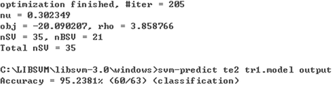
Linear kernel function experiment result
-
In Fig. 3, #iter is iterations; nu is the parameters of the selected kernel function type; Obj and rho are the minimum, which comes from the quadratic programming method and the decision function constant term, respectively; NSV, nBSV, and Total nSV are the support vector, boundary support vector, and the total number of support vectors, respectively. We can see from the experimental results of the linear kernel function that the model is made up of 35 support vectors from 205 iterations. Using the file tr1.model (tr1 as the training sample set) to classify and estimate 63 test samples, te2, and to output results systematically, namely, the classification accuracy of “Accuracy = 95.2381 %,” with a denominator of “60/63” representing the test sample number, the molecule represents the number in the test sample with correct classification.
-
-
Experiment 2
When the kernel function is the polynomial function (poly function), the experiment result is as shown in Fig. 4.
Fig. 4 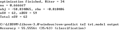
Polynomial Kernel function experiment result
-
The output shows that the iterations were 34 to finally obtain the tr1.model, and was composed of 62 support vectors. To use the test samples for testing the model generalization ability, we found that the model classification accuracy compared with other methods is the lowest one, only about 55.5556 %.
-
-
Experiment 3
When the kernel function is the radial basis function (RBF), the experiment result is as shown in Fig. 5.
Fig. 5 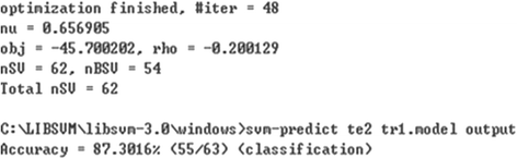
Radial basis kernel function experiment result
-
Figure 5 shows that using the RBF radial basis as kernel function to obtain the SVM model results in 48 iterative calculations, made up of 62 support vectors; the accuracy of using the file tr1.model to classify the 63 test samples was higher than the polynomial kernel function, with the classification accuracy of about 87.3016 %.
-
-
Experiment 4
When the nuclear function is the sigmoid kernel function, the experiment result is as shown in Fig. 6.
Fig. 6 
Multilayer perception kernel function experiment result
-
As shown in the output result for Fig. 6, when using the multilayer perception kernel function, the system only needs 35 iterative calculations to obtain the file tr1. model, composed of 62 support vectors; using the model file to classify 63 test samples, the classification accuracy was relatively low, only about 60.3175 %.
-
In the process of the SVM model construct, based on the differences in sample number and type, #iter and nSV will also change. The training results evaluation stage is meant to verify the model generalization ability, which is obtained from the training. Generalization ability refers to the adaptability of the machine learning algorithms for fresh samples. In the process of machine learning, the first step is to find the law hidden in the training sets of data. Then by using the same law of training sets of data, the SVM model can give appropriate output of testing sets of data. This kind of ability is called generalization ability. From the predicted results of the abovementioned four experiments, we found that the classification accuracy of the linear kernel function and the RBF function were higher. At the same time, the iterations of the different kernel functions, nSV, nBSV, and the effect of the parameters during training were not the same; the effects of the classified predictions are shown in Table 3.
Table 3 Comparison of the classification effects of the four kernel functions -
When using the linear function as the kernel function, with the algorithm convergence at 205 iterate steps, there are only 35 support vectors, which is the least of the four kernel functions. When using the polynomial as the kernel function, with the algorithm convergence at 34 iterate steps, there are 62 support vectors, but there are more boundary support vectors, vectors that are prone to interference. When using the RBF kernel function, the convergence speed is slightly slower than the polynomial function, but the number of support vectors is the same. However, there are 54 boundary support vectors, which is less than the polynomial function, and paranoid item b is close to 0; the sigmoid kernel function is similar to the polynomial kernel function, and therefore, an unfavorable selection.
-
The RBF kernel function has the following advantages. It can not only deal with nonlinear data (the linear kernel belongs to the special case of the RBF kernel) but also with parameter adjustment more concisely than the polynomial kernel due to its own hyperplane parameter. In addition, based on the preprocessing conditions of data during this analysis, these do not apply to sigmoid kernel function because there is no inner product of two vectors, and there appears to be invalid phenomenon for certain parameters. After considering all this, we chose to use the RBF kernel function as the inner kernel function of the SVM model as
-
$$ k\left({x}_i,x\right)={e}^{-\frac{{\left|x-{x}_i\right|}^2}{2{\sigma}^2}} $$(10)
-
Thus, the simulation experiment used here is the radial basis function as the kernel function for the SME credit risk evaluation model for SCF.
-
-
Experiment 1
-
-
(4)
Parameter optimization
-
Our analysis uses the method of cross-validation by toolkit LIBSVM to seek optimal parameters. Cross validation is a statistical analysis method used to verify the performance of the classifier. The basic idea of this method is as fellows. Firstly, we need to divide the original dataset into K groups. Secondly, each subset data should be as a validation set, while the rest of the K-1 subsets data as a training set. Then we can get K sets of model. Finally, the average classification accuracy of the K sets of model should be taken as the K - CV performance of the classifier. The most common method of cross-validation is the five-fold cross test. Here, we find the optimal parameters of RBF kernel function from easy.Py, which integrates with the module of grid.py, svm- train, svm-predict to realize the optimal parameter and the purpose of predicted classification. After input and debugging, the concluded optimal parameters are shown in Fig. 7.
Fig. 7 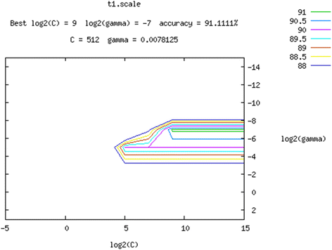
Fitting fig. of optimization result of parameters of RBF kernel function
-
Through optimizing selection, optimal parameters of RBF radial basis kernel function result in c = 512 and gamma = 0.0078125 after filtering, with these as the basic parameters to construct the SVM classification model.
-


Results and discussions
We used the optimization parameters found by the former crosscheck method to predict the test sample, with c =512, g = 0.0078125, and tr1.model base with the training sample data. The syntax is svm-train -c 512 -g 0.0078125 t1, and the output is shown in Fig. 8.

SVM classification based on credit risk assessment model prediction result
Comparison analysis of the SVM model and BP neural network model
Because sample learning enables the ability to incorporate a lot of uncertain information in a complex environment to judge complex issues, artificial neural network has been widely used for complex process estimations and predictions in recent years. Currently, there are numerous studies in which BP neural network algorithms have been applied to corporate financial crisis warnings and SME credit risk assessments, with the conclusion that the BP neural network is superior to traditional assessment methods. Therefore, this paper attempts to compare the classification results of the BP neural network model with the SVM model to explore the most effective model for SME credit risk assessment.
In the BP neural network model, the cross-validation method is used to achieve an optimal training model, with a target error of 0.0001, hidden layers of 15, the maximum number of training net.train.Param.epochs 10,000 times, and the training display interval net.train.Param.show set to1. The Matlab Neural Network Tool box provides a variety of training functions. Our analysis selected the most representative of the four algorithms, traingdx function, trainrp function, traincgp, and the trainscg function. We then selected the optimal one according to the experiment results. The results are shown in Table 4.
The results of the abovementioned training functions are shown in Fig. 9.

Chart of BP neural network training results with different training functions
The above mentioned comparison shows that the trainscg algorithm finally reached the standard of accuracy after 275 iterations. As the convergence speed was the fastest of the four algorithms, the trainscg algorithm was selected as the training function for our SME credit risk assessment model. Calling the training function net.trainFcnin Matlab = ‘trainscg’, we conducted a predicted classification on the test sample set. The classification results are shown in Table 5 below.
Table 5 classification results include the classification of the training sample and the classification of the test sample. If the Y value of sample enterprise data is −1 (non-creditworthy enterprise), but the classification model recognizes it as + 1 (creditworthy enterprise), then a TypeIerror in the model occurs. On the other hand, if sample enterprise data show its Y value as +1 and the classification model determines it as −1, then a Type II error occurs in the model. Altman noted that the loss induced by Type I errors is larger than the loss induced by Type II errors, which is almost 20 to 60 times greater (Altman 1980). Thus, in a single transaction, the loss that a bank may be subjected to from a Type I error is significantly higher. Therefore, we want to inspect the performance of a classification model considering not only the overall classification accuracy but also Type I errors.
Through the comparison of the results of the SVM and BP classification models, the SME credit risk assessment based on SVM from the perspective of SCF results in a high classification accuracy of 93.65 %, which is significantly higher than the classification accuracy of 55.56 % of the BP neural network. Therefore, from the view of the accuracy of the overall assessment, the SVM model is superior to the BP neural network model. This may be a result of high dimension and small size of the training sample. At the same time, the amount of data available for SCF is relatively scant due to the limited amount of SCF business during this timeframe. Thus, the SVM model is more practical when compared to the BP neural network model. On the other hand, despite the fact that the Type II error rate of the SVM model is higher than that of the BP neural network model, the Type I error rate of the SVM model is significantly lower than the BP neural network. Because it is more important for banks to reduce the Type I error rate to reduce losses, the SVM model is superior to the BP neural network model.
By comparing the classification results in Table 5, we can further analyze the robustness of the two models. In the training sample set, the accuracy of the SVM is higher than in the BP neural network; in the test sample set, the prediction accuracy of the SVM model increased by 2.79 %, while the prediction accuracy of the BP neural network declined by16.66 %. This showed us that the robustness of the BP neural network model was less than the SVM model. Furthermore, the results reflect that the learning generalization ability of the SVM model is superior to the BP neural network model. In addition, because the Type I error rate of the BP neural network model was 100 %, whereas the Type II error rate was 0, this implies that the BP neural network model can better identify the characteristics of the creditworthy enterprises, but cannot identify the characteristics of non-creditworthy enterprises. Such extreme classification results maybe because of the uneven distribution of the sample set and the limitations caused by the difficulty in collecting sample information. Because this problem cannot be avoided, the BP neutral network model is unsuitable for SCF bank credit risk evaluations.
Comparative analysis of two credit risk assessment index systems
The biggest difference between the traditional index system and the credit risk assessment index system designed here is that the supply chain leading enterprise’s credit status and the cooperative relationships between SMEs and leading enterprises are included in this designed index system. The traditional credit risk evaluation index system for SMEs comprises 19 indicators, as shown in Table 1, including aspects of industry conditions and SME credit status. We used the same sample with 153 enterprises to conduct the empirical research, and applied the two classification methods mentioned above under two types of index systems. The classification results are summarized in Table 6.
Through the results shown in Table 6, we find that the overall classification accuracy on the test sample of the SVM model is higher than in the BP neural network model, and that the accuracy of identifying non-creditworthy enterprises in the SVM model is considerably higher than in the BP neural network model. Through the comparison analysis presented in Tables 5 and 6, we also observe the following.
First, no change has occurred in the prediction accuracy of the BP neural network model, which indicates that the model did not have an insensitive reaction to dimension change. Therefore, there is little influence on the BP model’s classification accuracy when the index system changes. On the other hand, the SVM model had a positive reaction to dimension change. Consequently, the classification accuracy of the index utilized in this analysis is higher than in the traditional index system.
Second, the Type I error rate of the SVM model in Table 5 is far lower than that of the SVM model in Table 6, which indicates that the SCF credit risk assessment index system can aid commercial banks in reducing Type I error rates and reducing the probability of SME default behavior.
Third, the Type II error rate on the test sample of the SVM model in Table 5 is lower than that of the SVM model in Table 6,indicating that the SCF credit risk assessment index system can also aid commercial banks in reducing Type II error rates. Therefore, by comprehensively reflecting the SME credit status and cooperative relationships in the supply chain, the SCF credit risk assessment index system can help more SMEs to obtain funds.
Through the comprehensive comparison of Tables 5 and 6, we can understand the following.
-
(1)
The SCF credit risk assessment index system designed in this paper contained supply chain leading enterprise’s credit status and cooperative relationships between SMEs and leading enterprises can help banks to raise their accuracy on predicting a small and medium enterprise whether default or not. Therefore, more SMEs can obtain loans from banks through SCF.
-
(2)
The SCF credit risk assessment model based on SVM is of good generalization ability and robustness, which is more effective than BP neural network assessment model. Hence, Banks can raise the accuracy of credit risk assessment on SMEs by applying the SVM model, which can alleviate credit rationing on SMEs.
Therefore, the SCF credit risk assessment index system and the assessment model based on SVM, is the optimal combination for commercial banks to use to evaluate SMEs’ credit risk.
Conclusions
Main conclusions
Using the perspective of SCF, combined with the theory of supply chain management, an SCF credit risk assessment index system was designed. In this new index system, SMEs’ supply chain status, trade background, leading enterprises’ credit level, and the cooperative relationship between SMEs and leading enterprises are of great importance. And this new index can effectively reduce Type II error rates.
Furthermore, the SCF credit risk assessment index system can solve the problem of banks incorrectly labeling a creditworthy enterprise as a default enterprise, and thereby improve the credit rating status in the process of SME financing.
On the other hand, the classification accuracy of the SVM model is higher than the BP neural network model under the conditions of high dimension and small-sized sample. Moreover, the SVM model can efficiently reduce the probability of Type I errors under conditions where there is less historical data accumulation, but the dimensions of the assessment index have increased, and can thereby reduce the bank losses to a large extent.
In addition, besides classification accuracy, the robustness and learning generalization capacity of the SVM model is superior to the BP neural network model. Finally, combining the SCF credit risk assessment index system with SCF leads to a higher accuracy in predicting credit risk. Therefore, this combination is a better choice for commercial banks in addressing SCF credit risk management.
Limitations and further research
Although the SCF credit risk assessment model has superiority on predicting SMEs’ default behavior, but there are still some limitations in this model. Firstly, the size of total sample is limited. Because the SCF business become popular in recent years, there is no adequate accumulation of historical data on SCF. This limitation stop us from establishing a model which can carry out multilevel classification. Secondly, we cannot do a detailed discussion and research on different assessment model on different kind of SCF mode due to an insufficient sample data. Thirdly, the quantity of creditworthy enterprises’ questionnaires is more than non-creditworthy enterprises’ questionnaires. Because it is easier to obtain good credit enterprises’ information than bad credit enterprises, so there is data imbalance in the training sample set. Thus the data imbalance will cause the insufficient study on properties of default sample, which has bad effect on the classification accuracy of both SVM and BP model.
With the continuous development of supply chain finance business and the steady accumulation of relevant historical data, we want to do the further research in the following three aspects. On the one hand, we want to construct different credit risk assessment model according to different supply chain financing mode, including inventory mortgage, receivables pledge and purchase-order financing. On the other hand, we can establish multilevel classification model based on SVM to meet the banks’ demand of nine/ten-tier classification of loans. In addition, we will adjust the SCF credit risk assessment index according different industries. Because different industries have different characteristics. It is necessary to study how the supply chain relationships influence the SMEs’ credit risk in different industries.
References
Altman EI (1980) Commercial Bank Lending: Process, Credit Scoring and Costs of Errors in Lending. J Financial and Quantitative Analysis 15(4):813–832
Anderson JC, Håkansson H, Johanson J (1994) Dyadic Business Relationships within a Business Network Context. J Marketing 58(4):1–15
Atkinson, W. (2008) Supply Chain Finance: The Next Big Opportunity. J Supply Chain Management Review, 57-60
Chang K, Wang WH (2008) Financial service innovation—the risk analysis of warehouse receipt. J Modern Business 11:48–49
Chen CB, Sheng X (2013) A study of building risk evaluation system for supply chain financial credit. J Fujian Normal University (philosophy and social science edition) 02:22–86
Chen PY, Huang ZM (2002) SPSS10.0 statistical software application tutorial. People’s military medical press, Beijing
Cortes C, Vapnik V (1995) Support vector networks. J Machine Learning 20:273–297
Fan BN, Zhu WB (2003) Small and medium-sized enterprise credit evaluation index selection and the empirical analysis. J Scientific Research Management 24(6):83–88
Feldmann M, MÜller S (2003) An incentive scheme for true information providing in supply chains. Int J Management Science 31(2):63–73
Feng Y (2008) Supply chain financial: achieve multi-win-win situation of financial innovation service. J New Financial 2:60–63
Gupta S, Dutta K (2011) Modeling of financial supply chain. J European Journal of Operations Research 211:47–56
Hofmann, E. (2005). Supply Chain Finance: Some Conceptual Insights. In Lasch, R. /Janker, C.G. (Hrsg.): Logistik Management- Innovative Logistikkonzepte, Wiesbaden S: 203-214
Hu YF (2007) Supply chain financial: the new field which extremely rich potential. J China financial 22:38–39
Lewis, J. (2007) Demand Drives supply chain finance. J Treasury Perspectives, August: 20-23
Liu M, Lin DC (2005) Commercial bank credit risk assessment model based on support vector machine. J Xiamen university (natural science edition) 44(1):29–32
Mathis FJ, Cavinato J (2010) Financing the global supply chain: growing need for management action. J Thunderbird International Business Review 52(6):467–474
Pfohl HC, Gomm M (2009) Supply chain finance: optimizing financial flows in supply chains. J Logist Res 1:149–161
Silvestro R, Lustrato P (2014) Integrating financial and physical supply chains: the role of banks in enabling supply chain integration. Int J Operations & Production Management 34(3):298–324
Tang JR, Tan CH (2010) Research on the listed company credit risk assessment model based on support vector machine. J Statistics and Decision 10:65–67
Vapnik V (1995) The Natural of Statistical Learning Theory. Springer, New York
Walter A, Müller TA, Ritte T (2003) Functions of Industrial Supplier Relationships and Their Impact on Relationship Quality. J Industrial Marketing Management 32(2):159–169
Wan HD (2008) The analysis of supply chain financial model. J Economic Issues 11:109–111
Wang X, Wang H, Gong WH (2000) Principle and application of artificial neural network. Northeastern university press, Shenyang
West D (2000) Neural Network Credit Scoring Models. J Computers & Operations Research 27(11-12):1131–1152
Wu SB, Gu X (2008) A study of Cooperation relationship between knowledge chain organizations. J Management Science, and Science and Technology 2:113–118
Xiong X, Ma J, Zhao WJ (2009) Credit risk evaluation for supply chain finance mode. J Nankai Management Review 12(4):92–98
Yang YZ (2007) Theory of commercial bank supply chain finance risk prevention. J Financial BBS 10:42–45
Zhen T, Fan YF (2003) Research on enterprise credit risk assessment based on support vector machine (SVM). J Microelectronics and Computers 23(5):136–139
Zhou B (2010) Analysis for game theory of the risk of moral hazard for accounts receivable financing model. J Border Area, Economy and Culture 01:28–29
Acknowledgements
This research is sponsored by NSFC project (71372173、70972053); National Soft Science Research Project(2014GXS4D153); Specialized Research Fund of Ministry of Education for the Doctoral Project (20126118110017); Shaanxi Soft Science Research Project (2012KRZ13、2014KRM28-2、2013KRM08、2011KRM16); Shaanxi Social Science Funds projects (12D231, 13D217); Xi’an Soft Science Research Program (SF1225-2); Shaanxi Department of Education Research Project (11JK0175)、Shaanxi Department of Education Research Project (15JK1547);XAUT Teachers Scientific Research Foundation (107-211414).
Author information
Authors and Affiliations
Corresponding author
Additional information
Competing interests
The authors declare that they have no competing interests.
Authors’ contributions
Lang Zhang carried out the SCF credit risk assessment model based on SVM, and participated in the questionnaire design and drafted the manuscript. Haiqing Hu established the SCF credit risk assessment index system and helped to draft the manuscript. Dan Zhang participated in the design of the study and performed the statistical analysis. All authors read and approved the final manuscript.
Rights and permissions
Open Access This article is distributed under the terms of the Creative Commons Attribution 4.0 International License (http://creativecommons.org/licenses/by/4.0/), which permits unrestricted use, distribution, and reproduction in any medium, provided you give appropriate credit to the original author(s) and the source, provide a link to the Creative Commons license, and indicate if changes were made.
About this article

Cite this article
Zhang, L., Hu, H. & Zhang, D. A credit risk assessment model based on SVM for small and medium enterprises in supply chain finance. Financial Innovation 1, 14 (2015). https://doi.org/10.1186/s40854-015-0014-5
Received:
Accepted:
Published:
DOI: https://doi.org/10.1186/s40854-015-0014-5