Performance evaluation of series and parallel strategies for financial time series forecasting

Abstract

Background

Improving financial time series forecasting is one of the most challenging and vital issues facing numerous financial analysts and decision makers. Given its direct impact on related decisions, various attempts have been made to achieve more accurate and reliable forecasting results, of which the combining of individual models remains a widely applied approach. In general, individual models are combined under two main strategies: series and parallel. While it has been proven that these strategies can improve overall forecasting accuracy, the literature on time series forecasting remains vague on the choice of an appropriate strategy to generate a more accurate hybrid model.

Methods

Therefore, this study’s key aim is to evaluate the performance of series and parallel strategies to determine a more accurate one.

Results

Accordingly, the predictive capabilities of five hybrid models are constructed on the basis of series and parallel strategies compared with each other and with their base models to forecast stock price. To do so, autoregressive integrated moving average (ARIMA) and multilayer perceptrons (MLPs) are used to construct two series hybrid models, ARIMA-MLP and MLP-ARIMA, and three parallel hybrid models, simple average, linear regression, and genetic algorithm models.

Conclusion

The empirical forecasting results for two benchmark datasets, that is, the closing of the Shenzhen Integrated Index (SZII) and that of Standard and Poor’s 500 (S&P 500), indicate that although all hybrid models perform better than at least one of their individual components, the series combination strategy produces more accurate hybrid models for financial time series forecasting.

Background

Real time series forecasting with a high degree of accuracy is gaining increasing importance in many domains, particularly the financial markets, and thus, various attempts have been made to develop more accurate techniques. The objective of financial time series forecasting is to provide financial analysts and investors with reliable guidance on asset management. Thus, improving forecasting accuracy and introducing reliable forecasting methods can facilitate more profitable financial market investments by lead investors and financiers. To this effect, choosing a method that performs well in financial time series forecasting is imperative. To provide more accurate results, studies on time series forecasting and modeling widely use a combination of different models and metaheuristic optimization approaches. Considerable research has adopted optimization methods such as genetic algorithm (GA; Aghay Kaboli et al. 2016a, 2016b, Kaboli et al. 2016), particle swarm optimization (PSO; Aghay Kaboli et al. 2016a, 2016b), and gene expression programming (GEP; Aghay Kaboli et al. 2017a, 2017b; Aghay Kaboli et al. 2016a, 2016b). Kaboli et al. (2016) proposed the artificial cooperative search (ACS) algorithm to forecast long-term electricity energy consumption and numerically confirmed the effectiveness of the algorithm using other metaheuristic algorithms including the GA, PSO, and cuckoo search. Modiri-Delshad et al. (2016) presented a backtracking search algorithm (BSA) and verified the reliability of the method in solving and modeling the economic dispatch (ED) problem. Aghay Kaboli et al. (2016a, 2016b) estimated electricity demand using GEP, a genetic-based method, as an expression-driven approach and showed that GEP outperforms the multilayer perceptron neural (MLP) network and multiple linear regression models. Recent studies on time series forecasting largely focus on combination methods given the distinguishing features of hybrid models (e.g., unique modeling capability of each model), drawbacks in using single models, and the resultant improvements in forecasting accuracy. The key concept of combination theory is employing the unique merits of individual models to extract different data patterns. Importantly, the literature confirms that no individual model can universally determine data-generation processes. In other words, all characteristics of underlying data cannot be fully modeled by one model and therefore, combining different models or using hybrid ones helps analyze complex patterns in data more accurately and completely. Further, combining various models simplifies the selection of a model that is appropriate to process different forms of relationships in the data and reduces the risk of choosing an inefficient one.

Several approaches have been proposed to combine linear and nonlinear models. These combination methods are generally divided into two primary classes: series and parallel. In a series combination method, a time series is decomposed into linear and nonlinear parts. Accordingly, in the first stage, the model is used to process one time series component and then, the obtained values are used as inputs for the second model to analyze another component. On the other hand, in the parallel combination method, the original data are simultaneously considered to be inputs for different models and then, the linear combination of the forecasted results facilitates final hybrid forecasting.

The literature on series linear or nonlinear combination models has dramatically expanded since the early work of Zhang (2003). For instance, Pai and Lin (2005) proposed a series hybrid methodology to exploit the unique strength of autoregressive integrated moving average (ARIMA) and support vector machines (SVMs) to forecast stock price and indicated that a hybrid model outperforms its components. Chen and Wang (2007) constructed a series combination model that incorporates seasonal autoregressive integrated moving average (SARIMA) and SVMs for seasonal time series forecasting and achieved more accurate results than both components. Zeng et al. (2008) presented a series combination of the ARIMA and MLP models to predict short-term traffic flow. Their experimental results for the real datasets indicated that the proposed hybrid model can be an effective in improving forecasting accuracy achieved by either component. Zhou and Hu (2008) conducted experiments using a hybrid modeling and forecasting approach, which was based on the Grey and Box–Jenkins ARMA models, and showed that their proposed model had higher forecasting precision than its single components. Pao (2009) proposed a hybrid series model incorporating artificial neural network (ANN) and different types of generalized autoregressive conditional heteroscedasticity (GARCH) models to forecast energy consumption. Table 1 lists other recent studies on series linear and nonlinear hybrid models.

Table 1 Literature on series linear or nonlinear models for time series forecasting

Bates and Granger (1969) introduced the concept of a parallel combination, which was subsequently used by many researchers such as Makridakis et al. (1982), Granger and Ramanathan (1984), Bunn (1989), and De Menezes and Bunn (1993). Wedding and Cios (1996) proposed a parallel combination model using radial basis function networks and the Box–Jenkins ARIMA model. More recently, several parallel hybrid forecasting models have been proposed to combine linear and nonlinear models. For instance, Wang et al. (2012) presented a parallel hybrid model using GA and by employing ARIMA, exponential smoothing (ES), and back propagation neural network (BPNN) models. Their numerical results showed that the proposed model outperforms all traditional models, including the ESM, ARIMA, BPNN, equal weight hybrid (EWH) model, and random walk (RWM) model. Forecasting stock returns, Rather et al. (2015) proposed a novel hybrid model that merges predictions by three individual models: ES, recurrent neural network (RNN), and ARIMA; the optimum weights of each model are identified using GA. Yang et al. (2016) presented a combined forecasting model using BPNN, adaptive network-based fuzzy inference system (ANFIS), and SARIMA models, and thus, used a differential evolution metaheuristic algorithm to optimize the weights of a hybrid model. Their experimental case study showed that their proposed method performed better than the three individual methods and had higher accuracy.

In sum, several general conclusions can be drawn from the literature using hybrid models to explore time series forecasting. First, in recent years, there has a growing number of studies investigating the impact of using combination theory on forecasting accuracy; their objective is to enhance forecasting accuracy by combining different models. The numerical results of the reviewed papers evidence that the predictive capability and accuracy of hybrid models are better than those of single models. Moreover, hybrid models have recently become a dominated tool for time series forecasting. Second, scholars have introduced series and parallel combination methodologies to connect the components of hybrid models. However, the question of how to combine single models, that is, which combination yields more accurate results, remains unanswered. In other words, the literature has neglected to compare the two types of hybrid methods to introduce a more accurate one and focused on improving forecasting accuracy by employing hybrid models rather than their constituents. Third, the literature review revealed that among the linear and nonlinear models, ARIMA and MLPs have attracted overwhelming attention and perform well when part of hybrid models given their unique features. ARIMA models are one of the most important forecasting models that have been successfully applied in modeling and forecasting. The popularity of the ARIMA model can be attributed to its statistical properties and the well-known Box–Jenkins (Box and Jenkins 1976) methodology in the model-building process. The model assumes a linear correlation between the values of a time series and thus, performs well in linear modeling. MLP is the most well-known artificial neural network that processes nonlinear patterns in data without any assumption and does not require the determination of a model’s form. MLPs are flexible computing frameworks and universal approximators with a high degree of accuracy and can be applied to a wide range of forecasting problems. The key advantage of the neural networks is their flexible nonlinear modeling.

Given that the literature on time series forecasting remains ambiguous on the choice of combination strategy, the core objective of this study is to introduce an effective combination methodology and elucidate how individual models can be combined to improve financial time series forecasting. Accordingly, this study presents a comprehensive discussion on series and parallel combination methods and then, constructs a model using both techniques to combine MLP as a nonlinear model and ARIMA as a linear model. Then, using two combination strategies, ARIMA-MLP and MLP-ARIMA, the series and parallel hybrid models, comprising simple average (SA), linear regression (LR) and genetic algorithm (GA), are compared with their individual components. To evaluate the effectiveness of the hybrid models and introduce a more accurate and reliable hybrid method, two benchmark datasets, the closing of Shenzhen Integrated Index (SZII) and that of Standard and Poor’s 500 (S&P 500), are selected for the forecasting and modeling.

The remainder of this paper is organized as follows. Section Methods presents the basic concepts and modeling procedures of the ARIMA and MLP modes for time series forecasting. Section Series combination method of ARIMA and MLP models and Parallel combination of ARIMA and MLP describe the series and parallel combination techniques and the hybrid models constructed using these methods. Section Results and discussion reports the empirical results of the hybrid series and parallel models for a forecasting benchmark dataset. Section Comparison of forecasting results compares the performance of the models for the forecasting benchmark dataset. Section Conclusions concludes.

Methods

This section introduces the basic concepts and modeling procedures of the ARIMA and MLP models and series and the parallel hybrid methods for time series forecasting.

ARIMA model

ARIMA is one of the most widely used approaches to predict the future value of time series by extracting and modeling linear patterns in data. Therefore, the classic model is suitable for linear patterns. In ARIMA models, the future value of a variable is assumed to be a linear function of the past values and error terms.

$$ {y}_t={u}_t+{\upvarphi}_1{y}_{t-1}+\dots \dots +{\upvarphi}_p{y}_{t-p}-{\varepsilon}_t-{\theta}_1{\varepsilon}_{t-1}-\dots \dots -{\theta}_q{\varepsilon}_{t-q} $$

(1)

where (y _t ) is actual value in time t and ε _t is white noise, which is assumed to be independently and identically distributed with a mean of zero and constant variance of σ ² . p and q are the integer numbers of autoregressive and moving average terms in the ARIMA model and φ _i (i = 1,2,...., p) and θ _i (j = 1,2,....,q) are the model parameters to be estimated. The modeling procedure for the ARIMA models, which is based on the Box–Jenkins methodology, comprises three iterative steps: model identification, parameter estimation, and diagnostic checking. In the identification step, data transformation is often required to render the time series stationary, which is a necessary condition when building an ARIMA model for forecasting. A stationary time series is characterized by a constant mean and autocorrelation structure over time. When the observed time series presents a trend and heteroscedasticity, differencing and power transformation are applied to the data to remove the trend and stabilize the variance before the ARIMA model can be fitted. Once a tentative model is identified, the estimation of the model parameters is straightforward. The parameters are estimated such that an overall measure of errors is minimized, which can be accomplished using a nonlinear optimization procedure. The final step is the diagnostic checking of model adequacy, which determines if the model assumptions about errors a _t are satisfied.

Several diagnostic statistics and residual plots can be used to examine the goodness of fit of a tentatively adopted model to the historical data. If the model is deemed inadequate, a new tentative model is identified, which is also subjected to parameter estimation and model verification. Diagnostic information can help determine alternative model(s). This three-step model-building process is typically repeated several times until a satisfactory model is identified. The final model is then used for the prediction.

MLP model

Computational intelligence systems, more specifically, ANNs, which in fact, are a free dynamics model, are being widely used for the approximation of functions and forecasting. In the case of real-world problems, neural networks are an effective tool to recognize nonlinear patterns. ANNs are universal approximators that approximate a large class of functions with a high degree of accuracy, which is a crucial advantage over other classes of nonlinear models (Zhang et al. 1998). Their power is derived from the parallel processing of information from the data and no prior assumption is required in the model-building process. Instead, the network model is largely determined by the data characteristics. MLPs or single hidden layer feed-forward neural networks are key and commonly used model forms of ANNs for time series modeling and forecasting. The model is characterized by a network of three layers of simple processing units connected by acyclic links (Fig. 1). The relationship between the output (y _t ) and (y _t − 1, …, y _t − p ) inputs has the following mathematical representation (Khashei and Bijari 2010):

$$ {y}_t={w}_0+\sum \limits_{j=1}^q{w}_j\cdot g\left({w}_{0,j}+\sum \limits_{i=1}^p{w}_{i,j}\cdot {y}_{t-i}\right)+{\varepsilon}_t, $$

(2)

where w _{i, j} (i = 0,1,2,..., p, j = 1,2,...,q) and w _j (j = 0,1,2,...,q) are model parameters often termed connection weights, p is the number of input nodes, and q is the number of hidden nodes. The activation functions take several forms.

Fig. 1

MLP neural network architecture

The type of activation function is indicated by the condition of the neuron within the network. In a majority of cases, input layer neurons do not have an activation function because their role is to transfer inputs to the hidden layer. The most widely used activation function for the output layer is the linear function because a non-linear one may distort the predicated output. The logistic function is often used as a hidden layer transfer function, as shown in Eq. (3). Other activation functions can also be used such as linear and quadratic functions, each with a variety of modeling applications.

$$ Sig(x)=\frac{1}{1+\exp \left(-x\right)}. $$

(3)

Thus, the ANN model in Eq. (2) performs a nonlinear functional mapping from the past observations to the future value y, that is,

$$ {y}_t=f\left({y}_{t-1},\dots, {y}_{t-p},w\right)+{\varepsilon}_t, $$

(4)

where w is a vector of all parameters and f(.) is a function determined by the network structure and connection weights. Thus, the MLP is equivalent to a nonlinear autoregressive model. The simple network in Eq. (2) is unexpectedly powerful, that is, it can approximate the arbitrary function as a number of hidden nodes when q is sufficiently large. In practice, a simple network structure with a small number of hidden nodes often works well in out-of-sample forecasting, possibly because of the over-fitting effect typically found in the MLP modeling process. An over-fitted model has a good fit to the sample used for model building but poor generalizability to out-of-sample data.

The choice of q is data dependent and there is no systematic rule in deciding this parameter. In addition to choosing an appropriate number of hidden nodes, selecting the number of lagged observations, p, and dimensions of the input vector is an important task in the ANN modeling of a time series. This is, perhaps, the most important parameter to be estimated in an ANN model because it plays a major role in determining the (nonlinear) autocorrelation structure of the time series.

Series combination method of ARIMA and MLP models

In the series linear or nonlinear combination models, a time series is divided into a linear and nonlinear part, as follows:

$$ {y}_t=\sum \limits_{t=1}^n{L}_t+\sum \limits_{t=1}^n{N}_t $$

(5)

where L _t and N _t denote the linear and nonlinear parts estimated from the data. Then, these two components are sequentially processed by ARIMA and MLP models. Thus, in the first stage of this method, the ARIMA or MLP model is selected to identify linear or nonlinear patterns in the original data. Then, to discover the remaining patterns that are not captured by the first model, the output obtained in the first stage is used as an input for the second model. The basic concept is that one model is insufficient to capture all relationships in the data. Moreover, fully identifying and modeling the data characteristics in the real time series is difficult and sometimes, even impossible. Thus, using an individual model such as the ARIMA (MLP) model, undoubtedly, reveals nonlinear (linear) patterns that are not completely recognized. Consequently, the MLP (ARIMA) model is employed in the second stage to capture the remaining nonlinear (linear) patterns. A summation of the outputs obtained from the two stages is considered the final combined forecast. On the basis of the sequence of model selection, two hybrid models (ARIMA-MLP and MLP-ARIMA) are presented in the next section.

ARIMA-MLP model

In line with the series modeling procedure, in the first stage of the ARIMA-MLP model, the ARIMA is applied to model the linear component. Let e _t denote the residual of the ARIMA model at time t:

$$ {e}_t={y}_t-{\widehat{L}}_t $$

(6)

where ${\widehat{L}}_t$ is the forecasting value for time t from the ARIMA model based on original data. In the second stage, the residuals of the first stage are used as input data for the MLP model, allowing for the identification of nonlinear relationships. With n input nodes, the MLP model for the residuals will be.

$$ {e}_t=f\left({e}_{t-1},{e}_{t- 2},\dots, {e}_{t-n}\right)+{\varepsilon}_t\kern0.5em \Rightarrow \kern0.5em {{\widehat{N}}^{\prime}}_t={\widehat{e}}_t=f\left({e}_{t-1},{e}_{t-2},\dots, {e}_{t-n}\right) $$

(7)

where f is a nonlinear function determined by the MLP, ${{\widehat{N}}^{\prime}}_t$ is the forecasting value for time t in the MLP model based on residual data, and e _t is the random error. The framework for the ARIMA-MLP model is displayed in Fig. 2a.

Fig. 2

Framework of (a) ARIMA-MLP and (b) MLP-ARIMA model

Note that if model f is inappropriate, the error term is not necessarily random; therefore, the correct identification is critical. In this way, the combined forecast will be as follows:

$$ {\widehat{y}}_t=\widehat{L}{}_t+{{\widehat{N}}^{\prime}}_t $$

(8)

MLP-ARIMA model

Similar to the ARIMA-MLP model, the MLP-ARIMA model has two main stages. In the first stage, the MLP model is used to model the nonlinear part of the time series. Let ${e}_t^{\prime }$ denote the residual of the MLP model at time t. Then,

$$ {e}_t^{\prime }={y}_t-{\widehat{N}}_t $$

(9)

where ${\widehat{N}}_t$ is the forecasting value for time t in the MLP model based on the original data. Then, the residuals of MLP are stored as input of the ARIMA model. Accordingly, the ARIMA model with m lags for the residuals will be

$$ {e}_t^{\prime }=f\left({e}_{t-1}^{\prime },{e}_{t-2}^{\prime },\dots, {e}_{t-m}^{\prime}\right)+{\varepsilon}_t\kern0.5em \Rightarrow \kern0.5em {{\widehat{L}}^{\prime}}_t={{\widehat{e}}^{\prime}}_t=f\left({e}_{t-1}^{\prime },{e}_{t-2}^{\prime },\dots, {e}_{t-m}^{\prime}\right) $$

(10)

where f is a linear function determined by the ARIMA, ${{\widehat{L}}^{\prime}}_t$ is the forecasting value for time t in the ARIMA model on the residual data, and ε _t is the random error. The framework for the MLP-ARIMA model is displayed in Fig. 2b. Accordingly, the combined forecast is.

$$ {\widehat{y}}_t={{\widehat{L}}^{\prime}}_t+{\widehat{N}}_t $$

(11)

Parallel combination of ARIMA and MLP

In this method, the linear combination of the value forecasted by individual models is considered the output of a hybrid model and the desired weight of each component is calculated using different weighting approaches. In contrast to the series model, the original data are assigned to all individual models, after which the final forecast is obtained by multiplying each forecasted value with the desired weights. Suppose we select m individual models to generate hybrid forecasting. The linear combination of these models is as follows:

$$ {\widehat{y}}_t=\sum \limits_{i=1}^m{w}_i{\widehat{f}}_{it}\kern0.72em \left(t=1,\dots, n\right) $$

(12)

where ${\widehat{y}}_t\left(t=1,\dots, n\right)$ is the combined forecasting of actual data y _t (i = 1, …, n) at time t, ${\widehat{f}}_{it}\;\left(i=1,\dots, m\right)$ is the forecasting result obtained from the ith individual model at time t, m is the number of forecasting methods used to construct a hybrid model, and w _i is the weight of ith forecasting technique. The forecasting error of the hybrid model is calculated as follows:

$$ {e}_t={y}_t-{\widehat{y}}_t=\sum \limits_{i=1}^m{w}_i{y}_t-\sum \limits_{i=1}^m{w}_i{\widehat{f}}_{it}=\sum \limits_{i=1}^m{w}_i\left({y}_t-{\widehat{f}}_{it}\;\right)=\sum \limits_{i=1}^m{w}_i{e}_{it} $$

(13)

According to Eq. (9), the parallel combination of ARIMA and MLP is produced by Eq. (14):

$$ {\widehat{y}}_t={w}_1{\widehat{L}}_t+{w}_2{\widehat{N}}_t $$

(14)

where, ${\widehat{y}}_t$, ${\widehat{L}}_t$ and ${\widehat{N}}_t$ are the forecasting values which are obtained by hybrid, MLP and ARIMA models at time t respectively and w _i (i = 1, 2) is the weights allocated to each individual model. Thus the process modelling of this method is summarized in three steps:

• I. Modeling linear and nonlinear parts of time series using ARIMA and MLP models.

• II. Calculating weights of obtained values from the previous stage.

• III. Multiplying two desired weights coefficients to obtain forecasts from stage I and then summing them up.

Assigning the weights of each forecasting model is key to obtaining accurate forecasts using parallel methods because the weights indicate the importance and effectiveness of each individual component in a combined model. In addition, the forecasting results of a combined model with inappropriate weights may be less reliable than those of single models. The next section applies three well-known weighting approaches, SA, LR and GA, to develop three possible hybrid models.

Simple average-based hybrid model

Simple averaging is the easiest method in which equal weights are assigned to ARIMA and MLP, as shown in Eq. (15). However, in most cases, this method does not generate accurate forecasting results because it assumes that all forecasting models have a similar share in generating combined results or deals with forecasts as though they are exchangeable.

$$ {W}_1={W}_2=\frac{1}{2}\kern0.48em $$

(15)

Genetic algorithm-based hybrid model

A genetic algorithm is generally applied to solve optimization problems on the basis of a natural selection process that mimics biological evolution. The algorithm repeatedly modifies a population of individual solutions. At each step, the GA randomly selects individuals from the current population and uses them as parents to produce children for the next generation over successive generations; the population evolves toward an optimal solution. Given their ability to solve optimization problems, GAs are frequently used to determine optimum weights when using hybrid models.

Linear regression-based hybrid model

A regression method is commonly used to estimate parameters in different models such as weights in hybrid models. Eq. (16) is a linear regression that describes a dependent variable y _t  (t = 1, .…, n) using explanatory variables x _t (t = 1, .…, n), where k is the number of explanatory variables, β ₁, …, β _k and β ₀are the coefficients and intercept that must be estimated, and ε _t is the error term.

$$ {y}_t={\beta}_0+{\beta}_1{x}_{t1}+..\dots +{\beta}_k{x}_{tk}+{\varepsilon}_t $$

(16)

Using the ARIMA and MLP model as parts of a parallel hybrid model, two weights are estimated following the LR model:

$$ {y}_t={\beta}_0+{w}_1{\widehat{L}}_t+{w}_2{\widehat{N}}_t+{\varepsilon}_t $$

(17)

w ₁ and w ₂ are estimated using the ordinary least squares (OLS) approach, which minimizes the sum of the squared error between the actual value and final forecasting:

$$ \mathit{\operatorname{Min}}\;\sum \limits_{t=1}^n{\left({y}_t-{\widehat{y}}_t\right)}^2\kern0.36em $$

(18)

Then, β, w ₁ , and w ₂ are determined using the following equations:

$$ {\widehat{\beta}}_0={\overline{y}}_t-{\widehat{w}}_1{\overline{\widehat{L}}}_t-{\widehat{w}}_2{\overline{\widehat{N}}}_t $$

(19)

$$ {\widehat{w}}_1=\frac{\sum \limits_{t=1}^n{\widehat{N}}_t^2\sum \limits_{t=1}^n{\widehat{L}}_t{y}_t-\sum \limits_{t=1}^n{\widehat{L}}_t\widehat{N}\sum \limits_{t=1}^n\widehat{N}{y}_t}{\sum \limits_{t=1}^n{{\widehat{L}}_t}^2\sum \limits_{t=1}^n{\widehat{N}}_t^2-{\left(\sum \limits_{t=1}^n{\widehat{L}}_t{\widehat{N}}_t\right)}^2} $$

(20)

$$ {\widehat{w}}_2=\frac{\sum \limits_{t=1}^n{{\widehat{L}}_t}^2\sum \limits_{t=1}^n{\widehat{N}}_t{y}_t-\sum \limits_{t=1}^n{\widehat{L}}_t{\widehat{N}}_t\sum \limits_{t=1}^n{\widehat{L}}_t{y}_t}{\sum \limits_{t=1}^n{{\widehat{L}}_t}^2\sum \limits_{t=1}^n{{\widehat{N}}^2}_t-{\left(\sum \limits_{t=1}^n{\widehat{L}}_t{\widehat{N}}_t\right)}^2} $$

(21)

The key objective of this method is to capture the advantages of combining the ARIMA and MLP models in a linear and nonlinear pattern modeling for a time series forecast. The framework of the parallel hybrid models is illustrated in Fig. 3.

Fig. 3

Framework of parallel hybrid models

Results and discussion

This section applies the five hybrid models constructed using series and parallel combination strategies to forecast stock prices. To do so, the benchmark datasets Shenzhen Integrated Index (SZII) and S&P 500 are selected. Four error indicators, mean absolute error (MAE), mean squared error (MSE), mean absolute percentage error (MAPE), and root mean squared error (RMSE), are used for the evaluation and to rank the performance of the hybrid models, which are computed using the following equations. The dataset and modeling process for the hybrid models are presented in the next subsections.

$$ \mathrm{MAE}=\frac{1}{N}\sum \limits_{i=1}^N\left|{e}_i\right| $$

(22)

$$ MSE=\frac{1}{N}\sum \limits_{i=1}^N{\left({e}_i\right)}^2 $$

(23)

$$ MAPE=\frac{1}{N}\sum \limits_{i=1}^N\left(\frac{e_i}{y_i}\right) $$

(24)

$$ RMSE=\sqrt{\frac{1}{N}\sum \limits_{i=1}^N{\left({e}_i\right)}^2} $$

(25)

Shenzhen integrated index (SZII) dataset

The Shenzhen Integrated Index (SZII) dataset has a total of 216 monthly observations, spanning from January 1993 to December 2010 (Wang et al. 2012). The plot for the SZII dataset is presented in Fig. 4. According to previous studies, the first 168 observations (about 75% of the sample) are used as a training sample and the remaining 48 are applied as the test sample.

Fig. 4

Monthly SZII stock closing prices, January 1993–December 2010

ARIMA-MLP hybrid model

• Stage I - (Linear modeling): In the first stage of the ARIMA-MLP model, Eviews software is used, which identifies ARIMA(1, 0, 0)as the best fit. The stationary test (augmented Dickey–Fuller [ADF] Test) is applied to the SZII time series to test whether a unit root test exists in the ARIMA model. According to the obtained results, ADF test statistic is −3.676528 and the critical value of −3.432 is significant at the 5% level, the null hypothesis that a unit root test exists in the SZII time series is rejected.

• Stage II -(Nonlinear modelling): To analyze the obtained residuals from the previous stage and based on the concepts of MLP models, in MATLAB software, the best fitted model composed of four inputs, four hidden and one output neurons (in abbreviated form N ^{(4, 4, 1)}), is designed.

• Stage III - (Combination): In the final stage, the results obtained from stages I and II are combined. The estimated values of the ARIMA-MLP model against the actual values for all data are plotted in Fig. 5.

  Fig. 5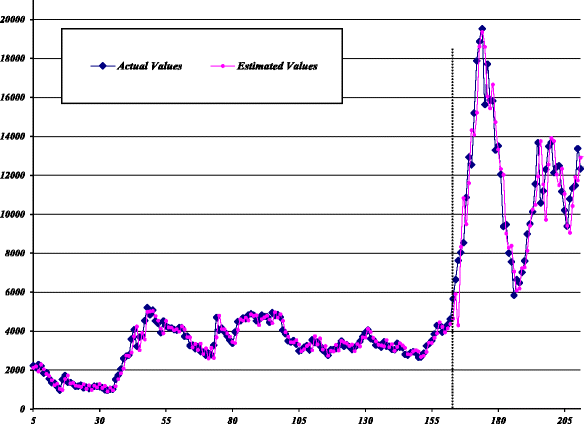

  

  Estimated values of ARIMA-MLP model for SZII

MLP-ARIMA hybrid model

• Stage I - (Nonlinear modeling): In the first stage of the MLP-ARIMA model, to capture the nonlinear patterns of a time series, an MLP with three input, two hidden, and one output neuron (abbreviated form: (N ^(3,2,1) )), is designed.

• Stage II - (Linear modeling): In the second stage of the MLP-ARIMA model, the residuals obtained from the previous stage are treated as the linear model. Thus, considering the lags of the MLP residuals as input variables of the ARIMA model, the best-fitted model is ARIMA(2, 0, 2).

• Stage III - (Combination): In the final stage, the results obtained from stages I and II are combined. The estimated values of the MLP-ARIMA model against the actual values for all data are plotted in Fig. 6.

  Fig. 6

  

  Estimated values of MLP-ARIMA model for SZII

Parallel hybrid models

Using SA, GA, and LR weighting approaches, the modeling procedure for the parallel hybrid models can be summarized in the following three steps.

• Stage I - (Linear and nonlinear modeling): Given the basic concepts of the ARIMA and MLP models in forecasting, the best-fit ARIMA and MLP models designed in Eviews and MATLAB software are ARIMA(1, 0, 0)and a one-layer neural network comprising three input, two hidden, and one output neuron (abbreviated form: (N ^(3,2,1) )). Note that different network structures are examined to compare MLP’s performance, and the structure hat reported the best forecasting accuracy for the test data is selected.

• Stage II - (Initializing weights): In this step, the optimum weights of the predicted values obtained from the previous stage are determined. Two weights are estimated by the LR model using the OLS approach in Eviews software, GA in MATLAB, and SA weighting approaches.

• Stage III - (Combination): In this stage, the final combined forecast is calculated by multiplying two optimal weight coefficients on the forecasts obtained from stage I and then, summing them up. The estimated values of the SA, GA, and LR-based hybrid models against the actual values are plotted in Figs. 7, 8, 9, respectively. The performance of the hybrid models and their components in the train and test datasets to forecast SZII are reported in Table 2. The table shows that, in both datasets, the MLP-ARIMA series model achieved higher prediction accuracy than the parallel and individual base models.

  Fig. 7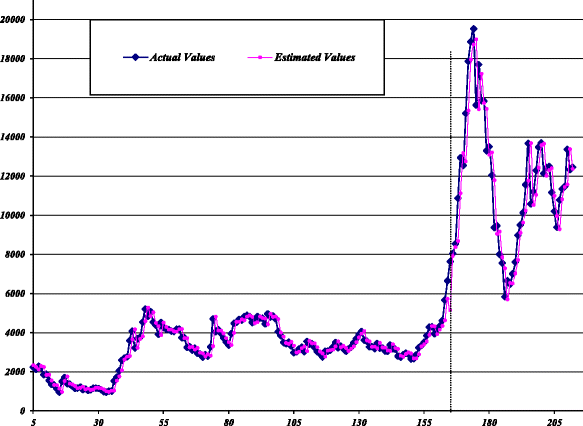

  

  Estimated values of SA-based hybrid model for SZII

  Fig. 8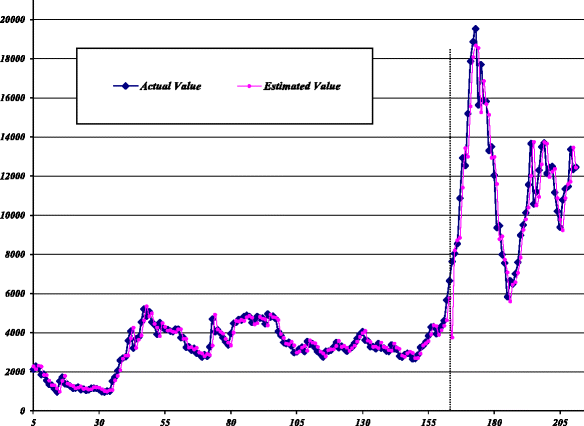

  

  Estimated values of GA-based hybrid model for SZII

  Fig. 9

  

  Estimated values of LR-based hybrid model for SZII

Table 2 Performance of models for SZII using train and test datasets

Standard and Poor’s 500 dataset

Standard and Poor’s 500 (S&P 500) dataset includes 2349 daily closing stock prices from October 1998 to February 2008 (Zhang and Wu 2009). The S&P 500 dataset is plotted in Fig. 10. According to previous studies, the S&P dataset is divided into training and test datasets. The first observations (about 80% of the sample) are used as the training sample to formulate the models and the last 470 observations are applied as a test sample to evaluate the performance of the constructed models.

Fig. 10

Daily S&P 500 stock closing prices, October 1998–February 2008

ARIMA-MLP series hybrid model

• Stage I - (Linear modeling): Similar to the linear modeling phase, ARIMA(1,0,0) is designed and the residuals of this step are used in the next step.

• Stage II - (Nonlinear modeling): In this stage, the residuals of the previous step are used as input for the MLP model and a network with three input, five hidden, and one output neuron is fitted to extract the remaining nonlinear structures.

• Stage III - (Combination): Here, the forecasted values of previous two stages are combined to generate the final combined forecast. The estimated values for the ARIMA-MLP model against the actual values for all data are plotted in Fig. 11.

  Fig. 11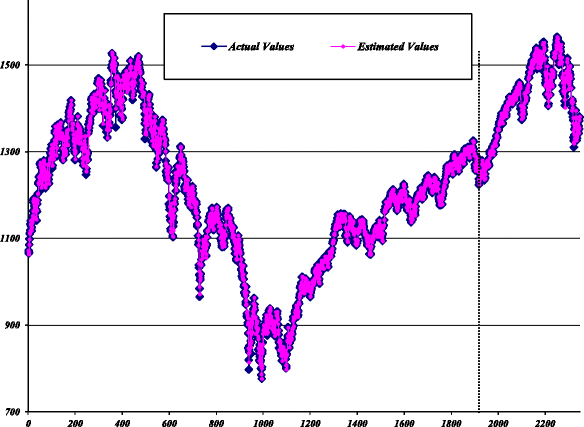

  

  Estimated values of ARIMA-MLP model for S&P 500

MLP-ARIMA series hybrid model

• Stage I - (Nonlinear modeling): In the nonlinear modeling phase, a network with three input, three hidden, and one output neurons is designed to capture the nonlinear relationships in the time series generated and the generated residuals are used in the next step.

• Stage II: (Linear modeling): In this step, an ARIMA (3, 0, 3) model is fit to process the linear structures that are not modeled by the MLP model.

• Stage III: (Combination): In the final step, the forecasted values from stages I and II are combined. The estimated values of the MLP-ARIMA model against the actual values for all data are plotted in Fig. 12.

  Fig. 12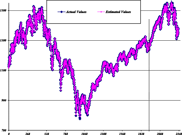

  

  Estimated values of MLP-ARIMA model for S&P500

Parallel hybrid models

• Stage I - (Linear and nonlinear modeling): Similar to the previous section, to capture the linear and nonlinear patterns in the data for the S&P time series, the ARIMA (1, 0, 0) and MLP models with three input, three hidden, and one output neuron are designed.

• Stage II - (Initializing weights): In this state, the optimum weights are derived by applying the LR, GA, and SA weighting methods. Note that the OLS approach and GA are designed using Eviwes and MATLAB software.

• Stage III - (Combination): According to the modeling procedure for the parallel hybrid models, the combined forecast is made using the values obtained from the previous two stages. The estimated values of the hybrid models based on parallel SA, GA, and LR against the actual values for all data are plotted in Figs. 13, 14, 15, respectively.

  Fig. 13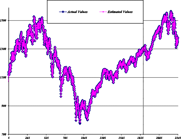

  

  Estimated values of SA-based hybrid model for S&P 500

  Fig. 14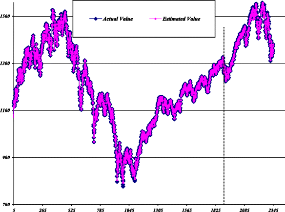

  

  Estimated values of GA-based hybrid model for S&P 500

  Fig. 15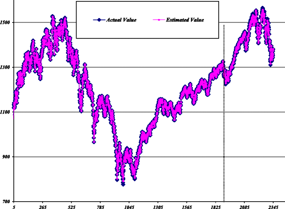

  

  Estimated values of LR-based hybrid model for S&P 500

Table 3 summarizes the performance of the series and parallel hybrid models in predicting the S&P 500 stock price using train and test datasets. The table shows that the series models, ARIMA-MLP and ARIMA-MLP, are not comparable with each other and reports significantly high prediction performance when the series hybrid methodology is used instead of the parallel methods and their base models.

Table 3 Performance of models for S&P 500 using train and test datasets

Comparison of forecasting results

This section compares the predictive capabilities of the hybrid models constructed by applying the series and parallel combination methods with either of their components, MLP, and ARIMA, using the two abovementioned datasets. The comparative analysis is conducted from two viewpoints: comparison of series and parallel hybrid models and analysis of average percentage improvement in the series and parallel hybrid models in comparison with their components. Two performance indicators, MAE and MSE, are employed to compare the forecasting performance of the hybrid models and their components.

In the first step, the overall performance of the series and parallel hybrid models is compared. Tables 4 and 5 present the overall performance of the hybrid models and their components for the SZII and S&P 500 datasets. The comparison reveals that the average forecasting error for MAE and MSE in the train and test datasets is lower in the ARIMA-MLP and MLP-ARIMA hybrid models constructed using the series combination technique than those in the parallel hybrid models. For example, in the SZII dataset, in MAE and MSE terms, the forecasting results of the series models using test dataset improved by 2.41% and 2.51% compared to those of the parallel hybrid models. Tables 4 and 5 compare the performance and accuracy of the series and parallel hybrid methods. In the second step, the performance of the hybrid models is compared with those of their base models. In other words, the average percentage improvement of the series and parallel hybrid models is compared with that of their base models. The results show that applying all five hybrid models, on average, improves the forecasting accuracy over at least one model for the ARIMA and MLP neural network models. This confirms the hypothesis that individual models do not capture all relationships in the data and combining the two models can be effective in overcoming their limitations and improving forecasting accuracy.

Table 4 Overall performance of series and parallel models for SZII

Table 5 Overall performance of series and parallel models for S&P 500

Tables 6 and 7 present the average improvement percentage of the series and parallel hybrid models for the SZII and S&P 500 datasets compared to the ARIMA and MLP models. The results suggest that, on average, the series hybrid models have a higher improving impact on the ARIMA and MLP models than the parallel hybrid models. For example, when using the S&P 500 dataset, the series hybrid models improve the MLP models in terms of MSE by 1.02% in the case of train data, while this improvement is −0.21 for the parallel models. According to the analytical results, the accuracies of the series hybrid models are better than those of the parallel hybrid models in both overall performance and average improvement percentage over the base models. From the above comparative analyses, the models can be ranked as follows: (i) series hybrid models (ii) parallel hybrid models, and (ii) individual models.

Table 6 Average improvement in series and parallel models over ARIMA and MLP models for SZII

Table 7 Average improvement in series and parallel models over ARIMA and MLP models for S&P 500

Conclusions

Forecasting real-world time series, particularly financial time series, is a critical task that has recently received overwhelming attention. Given the importance of accurate forecasting, several related methods have been proposed in the literature. In addition to single methods, studies have combined different methods to generate more accurate results and confirmed that combining different models enhances forecasting accuracy and accounts for the unique features of individual models. Although numerous studies have used series or parallel methods to construct hybrid models and confirm that combining different models reduces forecasting error and offer more accurate results, they remain vague on the precise combination that produces a more accurate hybrid model. Thus, this study proposed a more efficient technique to forecast financial time series and then, conducted a comprehensive comparison of the predictive capabilities of the series and parallel combination techniques that were combined with linear and nonlinear models, such as ARIMA and MLP, along with their individual components. First, the series and parallel hybrid models were compared, followed by a comparison of the hybrid models’ average percentage improvement with those of their base models. The empirical results for the two benchmark datasets, SZII and S&P 500, indicated that all hybrid models constructed using the two combination methods generated superior results than at least one of their individual components. The results also show that the series method generate more accurate hybrid models and has a higher improvement percentage than the parallel method. Therefore, the series combination method can be considered an efficient alternative to construct more accurate hybrid models in both analytical approaches to forecasting financial time series.

Future works should consider implementing the series and parallel hybrid methodologies to develop an approach with three or more individual models and accordingly, compare and analyze the obtained results. Researchers can also examine other statistical and intelligent models, such as GARCH and SVM models, to construct series and parallel hybrid models to forecast financial time series.

References

Adhikari R, Agrawal RK (2013) A combination of artificial neural network and random walk models for financial time series forecasting. J Neural Comput Appl 22:1–9
Aghay Kaboli SH, Selvaraj j, Rahim NA (2016a) Long-term electric energy consumption forecasting via artificial cooperative search algorithm. J Energy 115:857–871
Aghay Kaboli SH, Fallahpour A, Kazem N, Selvaraj J, Rahim NA (2016b) An expression-driven approach for long-term electric power consumption forecasting. J Data Min Knowl Discov 1(1):16–28
Aghay Kaboli SH, Selvaraj j, Rahim NA (2017a) Rain-fall optimization algorithm: a population based algorithm for solving constrained optimization problems. J Comput Sci 19:31–42
Aghay Kaboli SH, Fallahpour A, Selvaraj J, Rahim NA (2017b) Long-term electrical energy consumption formulating and forecasting via optimized gene expression programming. J Energy 126:144–164
Aladag CH, Egrioglu E, Kadilar C (2009) Forecasting nonlinear time series with a hybrid methodology. J Appl Math Lett 22:1467–1470
Barrow DK (2016) Forecasting intraday call arrivals using the seasonal moving average method. J Bus Res 69:6088–6096
Bates JM, Granger WJ (1969) The combination of forecasts. J Oper Res 20:451–468
Box P, Jenkins G (1976) Time series analysis: forecasting and control. Holden-day Inc, San Francisco, CA
Bunn D (1989) Forecasting with more than one model. J Forecasting 6:161–166
Chaâbane N (2014) A hybrid ARFIMA and neural network model for electricity price prediction. J Elec Pow Energy Syst 55:187–194
Chen KY, Wang CH (2007) A hybrid SARIMA and support vector machines in forecasting the production values of the machinery industry in Taiwan. J Expert Syst Appl 32:254–264
De Menezes L, Bunn D (1993) Diagnositic tracking and model specification in combined forecasts of U.K. inflation. J Forecasting 12:559–572
Ghasemi A, Shayeghi H, Moradzadeh M, Nooshyar M (2016) A novel hybrid algorithm for electricity price and load forecasting in smart grids with demand-side management. J Appl Energy 177:40–59
Granger CWJ, Ramanathan R (1984) Improved methods of combining forecasts. J Forecasting 3:197–204
Kaboli S H A; Fallahpour A, Kazemi N, Selvaraj J, Rahim N.A (2016) Electric energy consumption forecasting via expression-driven approach. 4th IET Clean Energy and Technology Conference
Katris C, Daskalaki S (2015) Comparing forecasting approaches for internet traffic. J Expert Syst Appl 42:8172–8183
Khashei M, Bijari M (2010) An artificial neural network (p, d, q) model for time series forecasting. J Exp Syst Appl 37:479–489
Khashei M, Bijari M, Raissi Ardali GA (2012) Hybridization of autoregressive integrated moving average (ARIMA) with probabilistic neural networks (PNNs). J Compu Indus Eng 63:37–45
Makridakis S, Andersen A, Carbone R, Fildes R, Hibon M, Lewandowski R, Wton J, Parzen E, Winkler R (1982) The accuracy of extrapolation (TimeSeries) methods: results of a forecasting competition. J Forecasting 1:111–153
Modiri-Delshad M, Aghay Kaboli SH, Taslimi-Renani E, Abd Rahim N (2016) Backtracking search algorithm for solving economic dispatch problems with valve-point effects and multiple fuel options. J Energy 116:637–649
Nourani V, Kisi O, Komasi M (2011) Two hybrid artificial intelligence approaches for modeling rainfall–runoff process. J Hydrol 402:41–59
Pai PF, Lin CS (2005) A hybrid ARIMA and support vector machines model in stock price forecasting. J Omega 33:497–505
Pao TH (2009) Forecasting energy consumption in Taiwan using hybrid nonlinear models. J Energy 34:1438–1446
Rather AM, Agarwal A, Sastry VN (2015) Recurrent neural network and a hybrid model for prediction of stock returns. J Exp Syst Appl 42:3234–3241
Wang X, Meng M (2012) A hybrid neural network and ARIMA model for energy consumption forecasting. J Comput Secur 7(5):1184–1190
Wang J-J, Wang J-Z, Zhang Z-G, Guo S-P (2012) Stock index forecasting based on a hybrid model. J Omega 40:758–766
Wedding DK II, Cios KJ (1996) Time series forecasting by combining RBF networks, certainty factors, and the box-Jenkins model. J Neuro-Oncol 10:149–168
Wu J, Chan CK (2011) Prediction of hourly solar radiation using a novel hybrid model of ARMA and TDNN. J Solar Energy 85:808–817
Yang Y, Chen Y, Wang Y, Li C, Li L (2016) Modelling a combined method based on ANFIS and neural network improved by DE algorithm: a case study for short-term electricity demand forecasting. J Appl Soft Comput 49:663–675
Zeng D, Xu J, Gu J, Liu L, Xu G (2008) Short term traffic flow prediction using hybrid ARIMA and ANN models. In: Power Electronics and Intelligent Transportation System, pp 621–625
Zhang GP (2003) Time series forecasting using a hybrid ARIMA and neural network model. J Neuro-Oncol 50:159–175
Zhang Y, Wu L (2009) Stock market prediction of S&P 500 via combination of improved BCO approach and BP neural network. J Exp Syst Appl 36:8849–8854
Zhang G, Patuwo BE, Hu MY (1998) Forecasting with artificial neural networks: the state of the art. J Int J Forecast 14:35–62
Zhou ZHJ, Hu C-H (2008) An effective hybrid approach based on grey and ARMA for forecasting gyro drift. J Chaos Solitons Fractals 35:525–529
Acknowledgements
The authors express their gratitude to Dr. Farimah Mokhatab Rafiei, associate professor of industrial engineering at the Tarbiat Modares University of Tehran, and Dr. Mehdi Bijari, professor of industrial engineering at Isfahan University of Technology, for their insightful and constructive comments, which have helped considerably improve this paper.
Funding
The authors have no funding to report.
Availability of data and materials
Not applicable.
Author information
Authors and Affiliations
Contributions
All authors have equally contributed to this work and approve of this submits.
Corresponding author
Ethics declarations
Competing interests
The authors declare that they have no competing interests.
Publisher’s Note
Springer Nature remains neutral with regard to jurisdictional claims in published maps and institutional affiliations.
Rights and permissions
Open Access This article is distributed under the terms of the Creative Commons Attribution 4.0 International License (http://creativecommons.org/licenses/by/4.0/), which permits unrestricted use, distribution, and reproduction in any medium, provided you give appropriate credit to the original author(s) and the source, provide a link to the Creative Commons license, and indicate if changes were made.
About this article
Cite this article
Khashei, M., Hajirahimi, Z. Performance evaluation of series and parallel strategies for financial time series forecasting. Financ Innov 3, 24 (2017). https://doi.org/10.1186/s40854-017-0074-9
Received:
Accepted:
Published:
DOI: https://doi.org/10.1186/s40854-017-0074-9